SparkNet : Training Deep Networks in Spark SPARKNET: TRAINING DEEP NETWORKS IN SPARK Training deep networks is a time-consuming process, with networks for object recognition often requiring multiple days to train. For this reason, leveraging the resources of a cluster to speed up training is an important area of work. However, widely-popular batch-processing computational frameworks like MapReduce and Spark were not designed to support the asynchronous and communication-intensive workloads of existing distributed deep learning systems. We introduce SparkNet, a framework for training deep networks in Spark. Our implementation includes a convenient interface for reading data from Spark RDDs, a Scala interface to the Caffe deep learning framework, and a lightweight multidimensional tensor library. Using a simple parallelization scheme for stochastic gradient descent, SparkNet scales well with the cluster size and tolerates very high-latency communication. Furthermore, it is easy to deploy and use with no parameter tuning, and it is compatible with existing Caffe models. We quantify the dependence of the speedup obtained by SparkNet on the number of machines, the communication frequency, and the cluster’s communication overhead, and we benchmark our system’s performance on the ImageNet dataset. Deep Networks를 학습시키는 것은 시간이 소요되는 프로세스로, 물체 인식(Object Recognition) 네트워크를 학습시키기 위해서는 며칠이 걸립니다. 이러한 이유로 클러스터의 자원을 활용하여 학습의 속도를 높이는 것은 작업의 중요한 분야였습니다. 그러나, 널리 사용되고 있는 맵 리듀스(MapReduce)나 Spark와 같은 일괄-처리(batch-processing) 계산 프레임 워크(framework)는 존재하는 분산 딥러닝 시스템의 비동기적(asynchronous)이고, 통신 집약적(communication-intensive)인 작업 부하를 지원하도록 설계되지 않습니다. SparkNet은 Spark에서 Deep Networks를 학습하기 위한 프레임워크입니다. Sparknet의 구현에는 Spark RDD에서 데이터를 읽을 수 있는 편리한 인터페이스와 Caffe 딥러닝 프레임 워크의 Scala 인터페이스와 경량화된 다차원 텐서(tensor) 라이브러리를 포함합니다. 간단한 병렬화 체계(Parallelization scheme)을 확률적 경사 하강(SGD : Stochastic Gradient Descent) 사용하는 SparkNet은 클러스터 크기에 맞춰 확장되며, 매우 높은 대기 시간(latency)의 통신을 지원합니다. 더욱더, 매개 변수 튜닝 없이 쉽게 배치하고 사용할 수 있으며, 존재하는 Caffe 모델과 호환됩니다. 다수의 머신으로 SparkNet을 통해 얻은 속도 향상과, 통신 빈도(communication frequency), 그리고 클러스터의 통신 오버헤드를 정량화하고, ImageNet 데이터셋의 시스템 성능을 벤치마크 하였습니다. * Spark https://spark.apache.org/docs/latest/ Apache Spark is a fast and general-purpose cluster computing system. It provides high-level APIs in Java, Scala, Python and R, and an optimized engine that supports general execution graphs. It also supports a rich set of higher-level tools including Spark SQL for SQL and structured data processing, MLlib for machine learning, GraphX for graph processing, and Spark Streaming. * Spark RDD : Resilient Distributed Datasets MapReduce에서 효율적인 Data Sharing 도구를 만들기 위해. HDFS를 거치지 말고, 용량이 넘쳐나는 RAM을 사용해보자. RAM을 이용하면 문제점은 중간에 Fault가 발생하면 어떻게 할 것인가? RAM을 사용하되, fault-tolerant & efficient한 RAM storage를 만들수 있을 것인가? 기존의 RAM을 쓰던 패러다임을 바꿔 Read-Only로 사용하여 해결을 한 것이 RDD이다. RDD의 특성으로는 Immutable(read-only), partitioned collections of records Deep learning has advanced the state of the art in a number of application domains. Many of the recent advances involve fitting large models (often several hundreds megabytes) to larger datasets (often hundreds of gigabytes). Given the scale of these optimization problems, training can be time consuming, often requiring multiple days on a single GPU using stochastic gradient descent (SGD). For this reason, much effort has been devoted to leveraging the computational resources of a cluster to speed up the training of deep networks (and more generally to perform distributed optimization). 딥 러닝은 많은 응용 분야에서 최첨단 기술을 발전 시켰습니다. 최근의 많은 발전은 더 큰 데이터 세트(종종 수백 기가 바이트)에 대형 모델(종종 수백 메가 바이트)을 맞추는 것을 포함합니다. 이러한 최적화 문제의 규모가 주어지면, 학습에 시간이 오래 걸릴 수 있으며 SGD를 사용하여 단일 GPU에서 운용할 경우 며칠을 필요로 하는 경우가 발생합니다. 이러한 이유 때문에 클러스터의 계산 리소스를 활용하여 심층 네트워크의 학습을 가속화 하는데 더 많은 노력을 기울여 왔습니다. (보다 일반적으로 분산 최적화를 수행하기 위해서) Many attempts to speed up the training of deep networks rely on asynchronous, lock-free optimization (Dean et al., 2012; Chilimbi et al., 2014). This paradigm uses the parameter server model (Li et al., 2014; Ho et al., 2013), in which one or more master nodes hold the latest model parameters in memory and serve them to worker nodes upon request. The nodes then compute gradients with respect to these parameters on a minibatch drawn from the local data shard. These gradients are shipped back to the server, which updates the model parameters. 딥 네트워크의 학습을 가속화하려는 많은 시도는 비동기식, 잠금 없는 최적화 lock-free optimization(Dean et al., 2012; Chilimbi et al., 2014)에 의존하였습니다. 이 패러다임 파라미터 서버 모델(Li et al., 2014; Ho te al., 2013)을 사용하였으며, 이는 하나 이상의 마스터 노드(master node)가 최신의 모델 파라미터(parameter)을 메모리에 보유하고, 요청시 작업 노드(worker nodE)에 제공하였습니다. 그런 다음 노드는 로컬 데이터(local data) 조각에서 가져온 미니 배치(mini batch)의 parameter로 Gradient를 계산합니다. 이러한 Gradient는 서버로 보내지며, 모델 parameter를 업데이트 하였습니다. At the same time, batch-processing frameworks enjoy widespread usage and have been gaining in popularity. Beginning with MapReduce (Dean & Ghemawat, 2008), a number of frameworks for distributed computing have emerged to make it easier to write distributed programs that leverage the resources of a cluster (Zaharia et al., 2010; Isard et al., 2007; Murray et al., 2013). These frameworks have greatly simplified many large-scale data analytics tasks. However, state-of-the-art deep learning systems rely on custom implementations to facilitate their asynchronous, communication-intensive workloads. One reason is that popular batch-processing frameworks (Dean & Ghemawat, 2008; Zaharia et al., 2010) are not designed to support the workloads of existing deep learning systems. SparkNet implements a scalable, distributed algorithm for training deep networks that lends itself to batch computational frameworks such as MapReduce and Spark and works well out-of-the-box in bandwidth-limited environments. 동시에, 일괄 처리 프레임 워크는 널리 사용되며 인기를 얻고 있습니다. MapReduce(Dean & Ghemawat, 2008)로 시작하여, 분산 컴퓨팅을 위한 여러 프레임 워크가 등장하였고, 클러스터의 자원을 활용하는 분산된 프로그램을 작성하는 것이 쉬워졌습니다. (Zaharia et al., 2010; Isard et al., 2007; Murray et al., 2013) 이러한 프레임 워크는 많은 대규모 데이터 분석 작업을 크게 단순화 시켰습니다. 그러나 최첨단 심층 학습 시스템은 비동기식(asynchronous), 통신 집약적인 작업 부하를 원할하기 위해 맞춤식 구현에 의존하게 되었습니다. 이러한 이유는 인기 있는 배치 처리 프레임 워크 (Dean & Ghemawat, 2008; Zaharia et al., 2010)가 기존의 심층 학습 시스템의 작업 부하를 지원하도록 설계되지 않았기 때문입니다. SparkNet은 MapReduce 및 Spark와 같은 일괄 계산 프레임 워크를 제공하고, 대역폭이 제한된 환경에서도 작동되는 Deep Network를 학습시키기 위해 확장 가능한 분산 알고리즘을 구현합니다. The benefits of integrating model training with existing batch frameworks are numerous. Much of the difficulty of applying machine learning has to do with obtaining, cleaning, and processing data as well as deploying models and serving predictions. For this reason, it is convenient to integrate model training with the existing data-processing pipelines that have been engineered in today’s distributed computational environments. Furthermore, this approach allows data to be kept in memory from start to finish, whereas a segmented approach requires writing to disk between operations. If a user wishes to train a deep network on the output of a SQL query or on the output of a graph computation and to feed the resulting predictions into a distributed visualization tool, this can be done conveniently within a single computational framework. 기존의 일괄 프레임워크와 모델 학습을 통합하면 많은 이점을 얻을 수 있습니다. 기계학습을 적용하는데는 데이터를 획득(obtaining), 가공(cleaning), 처리(processing)하는 것 뿐만 아니라, 모델을 배치하고, 예측을 제공하는데 많은 어려움이 있습니다. 이러한 이유로 오늘날의 분산형 시스템에서 설계된 기존 데이터 처리 파이프라인을 이용해 모델을 통합하는 것이 편리합니다. 또한 이러한 접근 방식을 사용하면 데이터를 처음부터 끝까지 메모리에 보관할 수 있지만, 세그먼트(segment) 방식에서는 작업간에 디스크에 쓰기가 필요합니다. 사용자가 SQL 쿼리의 출력이나 그래프 계산의 결과에 대한 딥 네트워크를 학습시키고, 결과 예측을 분산 시각화(visualization) 도구에서 제공하려는 경우, 이 작업은 단일 계산 프레임 워크 내에서 편리하게 수행할수 있습니다. We emphasize that the hardware requirements of our approach are minimal. Whereas many approaches to the distributed training of deep networks involve heavy communication (often communicating multiple gradient vectors for every minibatch), our approach gracefully handles the bandwidth-limited setting while also taking advantage of clusters with low-latency communication. For this reason, we can easily deploy our algorithm on clusters that are not optimized for communication. Our implementation works well out-of-the box on a five-node EC2 cluster in which broadcasting and collecting model parameters (several hundred megabytes per worker) takes on the order of 20 seconds, and performing a single minibatch gradient computation requires about 2 seconds (for AlexNet). We achieve this by providing a simple algorithm for parallelizing SGD that involves minimal communication and lends itself to straightforward implementation in batch computational frameworks. Our goal is not to outperform custom computational frameworks but rather to propose a system that can be easily implemented in popular batch frameworks and that performs nearly as well as what can be accomplished with specialized frameworks. 이러한 접근 방식은 하드웨어 요구 사항을 최소화되어 있음을 강조한다. 딥 네트워크의 분산된 트레이닝에 대한 많은 접근 방식은 무거운(heavy) 통신(종종 모든 minibatch를 위한 multiple Gradient vectors 통신)을 필요로 하지만, 우리의 접근은 낮은 대기 시간의 통신을 가지는 클러스터의 이점을 취하면서 대역폭이 제한된 설정을 적절하게 처리합니다. 이러한 이유로 통신에 최적화되지 않은 클러스터에 우리의 알고리즘을 쉽게 배포할 수 있습니다. 구현은 5개의 EC2 클러스터 노드에서 즉시 작동하며, 모델 매개 변수(하나의 worker당 수백 메가 바이트)를 알리고(broadcasting), 수집하는데 20초 정도 소요되며 단일 minibatch Gradient 계산을 하는데 2초가 소요됩니다.(AlexNet 용) 우리는 최소한의 의사소통(communication)이 필요한 SGC를 병렬 처리하는 간단한 알고리즘을 제공하고, 일괄 계산 프레임워크에서 직접 구현할 수 있도록 제공합니다. 우리의 목표는 맞춤형 계산 프레임워크를 능가하는 것이 아니라, 인기 있는 일괄 처리 프레임워크에서 쉽게 구현할 수 있는 시스템을 제안하는 것 뿐만 아니라, 전문화된 프레임워크로 수행할 수 있는 작업입니다. Here we describe our implementation of SparkNet. SparkNet builds on Apache Spark (Zaharia et al., 2010) and the Caffe deep learning library (Jia et al., 2014). In addition, we use Java Native Access for accessing Caffe data and weights natively from Scala, and we use the Java implementation of Google Protocol Buffers to allow the dynamic construction of Caffe networks at runtime. 여기서 우리는 SparkNet의 구현을 설명합니다. SparkNet은 Apache Spark(Zaharia et al., 2010)와 Caffe의 딥러닝 라이브러리 (Jia et al., 2014) 기반으로 빌드 업(build-up) 되었습니다. 또한 Java 네이티브 액세스(Java Native Access)를 사용하여 Caffe 데이터에 접근하며, Scala에 가중치를 부여하고, Java 를 사용하여 실행 시간(run-time)에 동적으로 Caffe 네트워크를 생성할 수 있도록 허락하는 Google 프로토콜 버퍼를 구현하였습니다. The Net class wraps Caffe and exposes a simple API containing the methods shown in Listing 1. The NetParams type specifies a network architecture, and the WeightCollection type is a map from layer names to lists of weights. It allows the manipulation of network components and the storage of weights and outputs for individual layers. To facilitate manipulation of data and weights without copying memory from Caffe, we implement the NDArray class, which is a lightweight multi-dimensional tensor library. One benefit of building on Caffe is that any existing Caffe model definition or solver file is automatically compatible with SparkNet. There is a large community developing Caffe models and extensions, and these can easily be used in SparkNet. By building on top of Spark, we inherit the advantages of modern batch computational frameworks. These include the high-throughput loading and preprocessing of data and the ability to keep data in memory between operations. In Listing 2, we give an example of how network architectures can be specified in SparkNet. In addition, model specifications or weights can be loaded directly from Caffe files. An example sketch of code that uses our API to perform distributed training is given in Listing 3. Net 클래스는 Caffe를 래핑하고, Listing 1에 표시된 메소드를 포함하는 간단한 API를 보여줍니다. NetParams 유형은 네트워크 아키텍처를 지정하고 WeightCollection의 타입은 layer 이름으로 weight의 리스트의 맵입니다. 네트워크 구성 요소와 개별 레이어에 대해 weight와 output을 저장소를 조작할 수 있도록 허락합니다. NDArray 클래스는 경량화 다차원 텐서(Tensor) 라이브러리 입니다. Caffe를 기반으로 하는 이점 중 하나는 Caffe 모델 정의 또는 해석하는 파일이 자동으로 호환된다는 것입니다. Caffe 모델과 확장 기능은 SparkNet에서 사용할 수 있습니다. Spark 위에 구축함으로써 현대 일괄 계산 프레임 워크의 장점을 이어받습니다. 여기에는 처리량이 많은 로딩과 데이터의 전처리 및 작업 간에 데이터를 메모리에 유지하는 기능이 포함됩니다. Listing 2에는 SparkNet에서 네트워크 아키텍처를 지정하는 방법에 대한 예제가 있습니다. 또한 Caffe 파일에서 모델 설정 또는 weight를 직접 로드 할 수 있습니다. API를 사용하여 분산 된 학습(training)을 수행하는 코드의 예가 Listing 3에 나와있다. To perform well in bandwidth-limited environments, we recommend a parallelization scheme for SGD that requires minimal communication. This approach is not specific to SGD. Indeed, SparkNet works out of the box with any Caffe solver. 대역폭이 제한된 환경에서 성능을 발휘하려면, 최소한의 통신 만 필요로하는 SGD의 병렬화 구성을 권장합니다. 이 접근법은 SGD 에만 국한되지 않습니다. 사실, SparkNet은 Caffe solver와 함께 즉시 사용할 수 있습니다. The parallelization scheme is described in Listing 3. Spark consists of a single master node and a number of worker nodes. The data is split among the Spark workers. In every iteration, the Spark master broadcasts the model parameters to each worker. Each worker then runs SGD on the model with its subset of data for a fixed number of iterations τ (we use τ = 50 in Listing 3) or for a fixed length of time, after which the resulting model parameters on each worker are sent to the master and averaged to form the new model parameters. We recommend initializing the network by running SGD for a small number of iterations on the master. A similar and more sophisticated approach to parallelizing SGD with minimal communication overhead is discussed in Zhang et al. (2015). 병렬화 계획은 Listing 3에 설명되어 있습니다. Spark는 단일 마스터 노드와 다수의 작업자 노드로 구성된다. 데이터는 Spark Worker 사이에서 분리됩니다. 모든 반복에서 Spark Master는 모델 매개 변수를 각 작업자에게 방송(broadcast)합니다. 그런 다음 각 작업자(Worker)는 일련의 반복 τ (Listing 3에서 τ = 50 사용) 또는 고정된 시간 동안 데이터의 하위 집합으로 모델에서 SGD를 실행하고 그 후에 각 작업자(Worker)의 결과 모델 매개 변수를 마스터(Master)에게 전송하며, 새로운 모델 매개 변수를 평균으로 형성하게 합니다. 마스터에서 적은 수의 반복에 대해 SGD를 실행하여 네트워크를 초기화하는 것이 추천합니다. Zhang 등은 최소한의 통신 오버 헤드로 SGD를 병렬화하는 간단하고 정교한 방법을 논의합니다. (2015). The standard approach to parallelizing each gradient computation requires broadcasting and collecting model parameters (hundreds of megabytes per worker and gigabytes in total) after every SGD update, which occurs tens of thousands of times during training. On our EC2 cluster, each broadcast and collection takes about twenty seconds, putting a bound on the speedup that can be expected using this approach without better hardware or without partitioning models across machines. Our approach broadcasts and collects the parameters a factor of τ times less for the same number of iterations. In our experiments, we set τ = 50, but other values seem to work about as well. 각 Gradient 계산을 병렬화하기 위한 표준 접근 방식은 Training 동안 수만 번 발생하는 모든 SGD업데이트 후에, 모델 파라미터(worker당 수백 MB, 총 GB)를 방송(Broadcast)과 수집해야 합니다. EC2 클러스터에서 각 브로드 캐스트 및 수집에는 약 20초가 걸리며, 더 나은 하드웨어나, 머신 간에 모델을 분할 없이는 이러한 접근보다 더 나은 속도 향상에 제한이 있습니다. 우리의 접근 방식은 동일한 반복 횟수 동안 τ 시간의 인자만큼 매개 변수를 방송하고 수집합니다. 우리의 실험에서는 τ = 50으로 설정했으며, 다른 값들도 마찬가지로 작용할 것입니다. We note that Caffe supports parallelism across multiple GPUs within a single node. This is not a competing form of parallelism but rather a complementary one. In some of our experiments, we use Caffe to handle parallelism within a single node, and we use the parallelization scheme described in Listing 3 to handle parallelism across nodes. Caffe는 단일 노드 내의 여러 GPU에서 병렬 처리를 지원합니다. 이것은 경쟁 방식의 경쟁이 아니라 오히려 보완적인 형태입니다. 일부 실험에서는 Caffe를 사용하여 단일 노드 내에서 병렬 처리를 처리하고, Listing 3에서 설명한 병렬화 체계를 사용하여 노드 간 병렬 처리를 처리합니다. In Section 3.2, we will benchmark the performance of SparkNet and measure the speedup that our system obtains relative to training on a single node. However, the outcomes of those experiments depend on a number of different factors. In addition to τ (the number of iterations between synchronizations) and K (the number of machines in our cluster), they depend on the communication overhead in our cluster S. In Section 3.1, we find it instructive to measure the speedup in the idealized case of zero communication overhead (S = 0). This idealized model gives us an upper bound on the maximum speedup that we could hope to obtain in a real-world cluster, and it allows us to build a model for the speedup as a function of S (the overhead is easily measured in practice). 3.2 절에서 SparkNet의 성능을 벤치마킹하고, 단일 노드에서의 학습(training)과 비교하여 시스템이 얻는 속도 향상을 측정합니다. 그러나 이러한 실험의 결과는 여러 가지 요인에 따라 달라집니다. τ (동기화 간의 반복 횟수)와 K (클러스터의 시스템 수)는 클러스터 S의 통신 오버 헤드에 따라 달라집니다. 3.1 절에서 이상화 된 시스템의 속도 향상을 측정하는 것이 유용하다는 것을 알 수 있습니다. 통신 오버 헤드가 0인 경우 (S = 0), 이상적인 모델은 실제 클러스터에서 얻을 수있는 최대 속도 향상에 대한 상한선을 제공하며, S의 기능으로 속도 향상 모델을 구축 할 수 있습니다 (실제 오버 헤드는 쉽게 측정됩니다) Before benchmarking our system, we determine the maximum possible speedup that could be obtained in principle in a cluster with no communication overhead. We determine the dependence of this speedup on the parameters τ (the number of iterations between synchronizations) and K (the number of machines in our cluster). 시스템을 벤치마킹하기 전에, 우리는 통신 오버 헤드가 없는 클러스터에서 원칙적으로 얻을 수있는 최대 속도 향상으로 결정하였습니다. 이 속도 향상의 매개 변수 τ (동기화 간 반복 횟수)와 K (클러스터의 시스템 수)에 대한 의존성을 결정합니다. To begin with, we consider the theoretical limitations of a naive parallelism scheme which parallelizes SGD by distributing each minibatch computation over multiple machines (see Figure 2b). Let Na(b) be the number of serial iterations of SGD required to obtain an accuracy of a when training with a batch size of b (when we say accuracy, we are referring to test accuracy). Suppose that computing the gradient over a batch of size b requires C(b) units of time. Then the running time required to achieve an accuracy of a with serial training is Na(b)C(b). 우선, 여러 머신에 대해 각 minibatch 계산을 분산하여 SGD를 병렬화하는 naive parallelism scheme 의 이론적인 한계를 고려합니다 (그림 2b 참조). 일괄 처리 크기가 b 인 정확도(accuracy)를 얻기 위해 필요한 SGD의 순차 반복 수를 Na(b)로 지정합니다. (정확도를 말할 때는 테스트 정확도를 나타냅니다.) 크기 b의 배치에 대한 Gradient 계산에 C(b) 시간 단위가 필요하다고 가정합니다. 그런 다음 직렬 훈련의 정확도를 얻는 데 필요한 실행 시간은 Na(b)C(b)입니다. A naive parallelization scheme attempts to distribute the computation at each iteration by dividing each minibatch between the K machines, computing the gradients separately, and aggregating the results on one node. Under this scheme, the cost of the computation done on a single node in a single iteration is C(b/K) and satisfies C(b/K) ≥ C(b)/K (the cost is sublinear in the batch size). In a system with no communication overhead and no overhead for summing the gradients, this approach could in principle achieve an accuracy of a in time Na(b)C(b)/K. This represents a linear speedup in the number of machines (for values of K up to the batch size b). Naive 병렬화 계획은 K 머신간에 각 minibatch를 나누고, Gradient을 개별적으로 계산하고, 결과를 하나의 노드에 집계하여 각 반복마다 계산을 분산하려고 시도합니다. 이 계획에서 단일 반복에서 단일 노드에서 수행 된 계산의 비용은 C (b / K)이고 C (b / K) ≥ C (b) / K를 만족합니다 (비용은 배치 크기에서 sublinear 입니다) . 통신 오버 헤드가없고 Gradient를 합산하기위한 오버 헤드가 없는 시스템에서 이 접근법은 원칙적으로 시간 Na (b)C(b)/K의 정확도를 달성 할 수 있습니다. 이것은 기계 수의 선형 속도 증가를 나타냅니다 (배치 크기 b까지의 K 값). In practice, there are several important considerations. First, for the approximation C(b/K) ≈ C(b)/K to hold, K must be much smaller than b, limiting the number of machines we can use to effectively parallelize the minibatch computation. One might imagine circumventing this limitation by using a larger batch size b. Unfortunately, the benefit of using larger batches is relatively modest. As the batch size b increases, Na(b) does not decrease enough to justify the use of a very large value of b. 실제로는 몇 가지 중요한 고려 사항이 있습니다. 첫째, 근사값 C (b / K) ≈ C (b) / K를 유지하기 위해서는 K가 b보다 훨씬 작아야하므로 minibatch 계산을 효과적으로 병렬 처리 할 수 있는 기계의 수를 제한합니다. 더 큰 배치 크기 b를 사용하면이 한계를 우회 할 수 있습니다. 불행히도, 더 큰 배치를 사용하는 이점은 상대적으로 적습니다. 배치 크기 b가 증가함에 따라, Na(b)는 b의 매우 큰 값의 사용을 정당화하기에는 충분히 감소하지 않습니다. Furthermore, the benefits of this approach depend greatly on the degree of communication overhead. If aggregating the gradients and broadcasting the model parameters requires S units of time, then the time required by this approach is at least C(b)/K + S per iteration and Na(b)(C(b)/K + S) to achieve an accuracy of a. Therefore, the maximum achievable speedup is C(b)/(C(b)/K + S) ≤ C(b)/S. We may expect S to increase modestly as K increases, but we suppress this effect here. 더욱더, 이 접근 방식의 이점은 통신 오버 헤드의 정도에 크게 의존합니다. Gradient를 모으고 모델 파라미터를 브로드 캐스팅하는 데 S 단위 시간이 필요한 경우, 이 방법에 필요한 시간은 반복 당 최소 C(b)/K + S이며 Na(b) (C(b)/K + S) 의 정확성을 달성하기 위해. 그러므로 달성 가능한 최대 속도 증가는 C(b) / (C b)/K + S) ≤ C(b)/S이다. K가 증가함에 따라 S가 완만하게 증가 할 것으로 예상 할 수 있지만 여기에서는이 효과를 억제합니다. (a) This figure depicts a serial run of SGD. Each block corresponds to a single SGD update with batch size b. The quantity Na(b) is the number of iterations required to achieve an accuracy of a. (a) 이 그림은 SGD의 연속 실행을 보여줍니다. 각 블록은 배치 크기가 b 인 단일 SGD 업데이트에 해당합니다. Na(b)의 양은 a의 정확도를 달성하는 데 필요한 반복 횟수입니다. (b) This figure depicts a parallel run of SGD on K = 4 machines under a naive parallelization scheme. At each iteration, each batch of size b is divided among the K machines, the gradients over the subsets are computed separately on each machine, the updates are aggregated, and the new model is broadcast to the workers. Algorithmically, this approach is exactly equivalent to the serial run of SGD in Figure 2a and so the number of iterations required to achieve an accuracy of a is the same value Na(b). (b) 이 그림은 Naive 병렬화 체계 하에서 K = 4 시스템에서 SGD의 병렬 실행을 보여줍니다. 매 반복마다 크기 b의 각 배치가 K 시스템으로 나누어지고 각 시스템에서 부분 집합에 대한 Gradient가 개별적으로 계산되고 업데이트가 집계되며, 새 모델이 Worker에게 브로드 캐스팅됩니다. 알고리즘 적으로이 접근법은 그림 2a의 SGD의 직렬 실행과 정확히 동일하므로 a의 정확도를 달성하는 데 필요한 반복 횟수는 동일한 값 Na (b)입니다. (c) This figure depicts a parallel run of SGD on K = 4 machines under SparkNet’s parallelization scheme. At each step, each machine runs SGD with batch size b for τ iterations, after which the models are aggregated, averaged, and broadcast to the workers. The quantity Ma(b, K, τ ) is the number of rounds (of τ iterations) required to obtain an accuracy of a. The total number of parallel iterations of SGD under SparkNet’s parallelization scheme required to obtain an accuracy of a is then τMa(b, K, τ ). (c) 이 그림은 SparkNet의 병렬화 체계에서 K = 4 컴퓨터에서 SGD를 병렬 실행하는 것을 보여줍니다. 각 단계에서 각 시스템은 τ 반복을위한 배치 크기 b로 SGD를 실행 한 후 모델을 집계하고 평균을내어 Worker에게 브로드 캐스팅합니다. 수량 Ma (b, K, τ)는 a의 정확도를 얻기 위해 필요한 라운드 수 (τ 반복 수)입니다. 다음의 정확도를 얻기 위해 필요한 SparkNet의 병렬화 체계에서의 SGD의 병렬 반복 총 횟수는 τMa (b, K, τ)입니다. The performance of the naive parallelization scheme is easily understood because its behavior is equivalent to that of the serial algorithm. In contrast, SparkNet uses a parallelization scheme that is not equivalent to serial SGD (described in Section 2.1), and so its analysis is more complex. Navie parallelization scheme 의 성능은 serial 알고리즘의 동작과 동일하기 때문에 쉽게 이해할 수 있습니다. 반대로 SparkNet은 serial SGD (2.1 절에서 설명)와 동일하지 않은 병렬 처리 체계를 사용하므로 분석이 더 복잡합니다. SparkNet’s parallelization scheme proceeds in rounds (see Figure 2c). In each round, each machine runs SGD for τ iterations with batch size b. Between rounds, the models on the workers are gathered together on the master, averaged, and broadcast to the workers. SparkNet의 병렬 처리 계획은 라운드에서 진행됩니다 (그림 2c 참조). 각 라운드에서 각 시스템은 배치 크기가 b 인 τ 반복에 대해 SGD를 실행합니다. 라운드 사이에, Worker에 대한 모델이 마스터(Master)에 모여 평균화되어 Worker에게 방송됩니다. We use Ma(b, K, τ ) to denote the number of rounds required to achieve an accuracy of a. The number of parallel iterations of SGD under SparkNet’s parallelization scheme required to achieve an accuracy of a is then τMa(b, K, τ ), and the wallclock time is (τC(b) + S)Ma(b, K, τ ), (2) where S is the time required to gather and broadcast model parameters. Ma (b, K, τ)를 사용하여 a의 정확도를 달성하는 데 필요한 라운드 수를 나타냅니다. S의 정확도를 달성하는 데 필요한 SparkNet의 병렬화 체계에서 SGD의 병렬 반복 수는 τMa (b, K, τ)이고 wallclock 시간은 (τC (b) + S) Ma (b, K, τ) , (2) 여기서 S는 모형 매개 변수를 모으고 브로드 캐스트 하는데 필요한 시간이다. To measure the sensitivity of SparkNet’s parallelization scheme to the parameters τ and K, we consider a grid of values of K and τ . For each pair of parameters, we run SparkNet using a modified version of AlexNet on a subset of ImageNet (the first 100 classes each with approximately 1000 data points) for a total of 20000 parallel iterations. For each of these training runs, we compute the ratio τMa(b, K, τ )/Na(b). This is the speedup achieved relative to training on a single machine when S = 0. In Figure 3, we plot a heatmap of the speedup given by the SparkNet parallelization scheme under different values of τ and K. 매개 변수 τ와 K에 대한 SparkNet의 병렬화 체계의 민감도를 측정하기 위해 K와 τ의 값 표를 고려합니다. 각 쌍의 매개 변수에 대해 ImageNet의 하위 집합 인 AlexNet의 수정 된 버전 (약 1000 개의 데이터 요소가 있는 100 개의 클래스)을 사용하여 SparkNet을 실행하여 총 20000 개의 병렬 반복을 수행합니다. 이러한 각각의 훈련 실행에 대해 우리는 비율 τMa (b, K, τ) / Na (b)를 계산한다. 이것은 S = 0 일 때 단일 기계에 대한 교육에 비해 달성 된 속도 증가입니다. 그림 3에서는 SparkNet 병렬화 체계에서 주어진 τ와 K의 다른 값에 따른 속도 향상의 히트 맵을 그립니다. Figure 3: This figure shows the speedup τMa(b, τ, K)/Na(b) given by SparkNet’s parallelization scheme relative to training on a single machine to obtain an accuracy of a = 20%. Each grid square corresponds to a different choice of K and τ . We show the speedup in the zero communication overhead setting. This experiment uses a modified version of AlexNet on a subset of ImageNet (100 classes each with approximately 1000 images). Note that these numbers are dataset specific. Nevertheless, the trends they capture are of interest. 그림 3 :이 그림은 a = 20 %라는 정확도를 얻기 위해 SparkNet의 병렬화 기법이 단일 기계에서의 교육에 비해 주어진 속도 향상 τMa (b, τ, K) / Na(b)를 보여줍니다. 각 격자 사각형은 K와 τ의 다른 선택에 해당합니다. 우리는 제로 통신 오버 헤드 설정에서 속도 향상을 보여줍니다. 이 실험에서는 ImageNet의 하위 집합 인 AlexNet의 수정 된 버전을 사용합니다 (각각 약 1000 개의 이미지가있는 100 개의 클래스). 이 숫자는 데이터 세트별로 다릅니다. 그럼에도 불구하고 그들이 수집하는 경향은 중요합니다. Figure 3 exhibits several trends. The top row of the heatmap corresponds to the case K = 1, where we use only one worker. Since we do not have multiple workers to synchronize when K = 1, the number of iterations τ between synchronizations does not matter, so all of the squares in the top row of the grid should behave similarly and should exhibit a speedup factor of 1 (up to randomness in the optimization). The rightmost column of each heatmap corresponds to the case τ = 1, where we synchronize after every iteration of SGD. This is equivalent to running serial SGD with a batch size of Kb, where b is the batchsize on each worker (in these experiments we use b = 100). In this column, the speedup should increase sublinearly with K. We note that it is slightly surprising that the speedup does not increase monotonically from left to right as τ decreases. Intuitively, we might expect more synchronization to be strictly better (recall we are disregarding the overhead due to synchronization). However, our experiments suggest that modest delays between synchronizations can be beneficial. 그림 3은 몇 가지 경향을 보여줍니다. 히트 맵의 맨 위 줄은 K = 1 인 경우에 해당합니다. 여기서 우리는 단 하나의 Worker 만 사용합니다. K = 1 일 때 동기화 할 작업자가 여러 명 없으므로 동기화 간의 반복 횟수 τ는 중요하지 않으므로 그리드의 맨 위 행에있는 모든 사각형은 유사하게 동작해야 하며 1의 속도 향상 요소를 나타냅니다 (위로 최적화에서 임의성으로). 각 히트 맵의 가장 오른쪽 열은 SGD가 반복 될 때마다 동기화되는 τ = 1에 해당합니다. 이것은 배치 크기가 Kb 인 직렬 SGD를 실행하는 것과 같습니다. 여기서 b는 각 작업자의 배치 크기입니다 (이 실험에서는 b = 100을 사용합니다). 이 칼럼에서 속도 향상은 K와 함께 선형적으로 증가해야합니다. 우리는 속도 향상이 τ가 감소함에 따라 왼쪽에서 오른쪽으로 단조롭게 증가하지 않는다는 것이 약간 놀랍습니다. 직관적으로, 더 많은 동기화가 엄격하게 더 나은 것으로 기대할 수 있습니다 (동기화로 인한 오버 헤드를 무시함). 그러나 우리의 실험은 동기화 간의 적절한 지연이 유용 할 수 있음을 제시합니다. This experiment capture the speedup that we can expect from the SparkNet parallelization scheme in the case of zero communication overhead (the numbers are dataset specific, but the trends are of interest). Having measured these numbers, it is straightforward to compute the speedup that we can expect as a function of the communication overhead. 이 실험은 통신 오버 헤드가 없는 경우 SparkNet 병렬화 계획에서 기대할 수있는 속도 향상을 포착합니다 (이 수치는 특정 데이터 세트이지만 경향은 중요합니다). 이 수를 측정하면 통신 오버 헤드(overhead)의 함수로 예상 할 수있는 속도 향상을 계산하는 것이 간단합니다. Figure 4: This figure shows the speedups obtained by the naive parallelization scheme and by SparkNet as a function of the cluster’s communication overhead (normalized so that C(b) = 1). We consider K = 5. The data for this plot applies to training a modified version of AlexNet on a subset of ImageNet (approximately 1000 images for each of the first 100 classes). The speedup obtained by the naive parallelization scheme is C(b)/(C(b)/K + S). The speedup obtained by SparkNet is Na(b)C(b)/[(τC(b) + S)Ma(b, K, τ )] for a specific value of τ . The numerator is the time required by serial SGD to achieve an accuracy of a, and the denominator is the time required by SparkNet to achieve the same accuracy (see Equation 1 and Equation 2). For the optimal value of τ , the speedup is maxτ Na(b)C(b)/[(τC(b) + S)Ma(b, K, τ )]. To plot the SparkNet speedup curve, we maximize over the set of values τ ∈ {1, 2, 5, 10, 25, 100, 500, 1000, 2500} and use the values Ma(b, K, τ ) and Na(b) from the experiments in the fifth row of Figure 3. In our experiments, we have S ≈ 20s and C(b) ≈ 2s. 그림 4 : 이 그림은 클러스터의 통신 오버 헤드 (C(b) = 1이되도록 정규화 됨)의 함수로 Naive 병렬화 체계와 SparkNet에서 얻은 속도 향상을 보여줍니다. 우리는 K = 5를 고려합니다.이 플롯의 데이터는 ImageNet의 하위 집합인 AlexNet의 수정 된 버전을 학습하는 데(training) 적용됩니다 (처음 100 개 클래스 각각에 약 1000 개의 이미지). Naive 병렬화 기법으로 얻는 속도 향상은 C(b) / (C(b) / K + S)입니다. SparkNet이 얻는 속도 향상은 τ의 특정 값에 대해 Na(b) C(b) / [(τC(b) + S) Ma(b, K, τ)]입니다. 분자는 a의 정확도를 얻기 위해 직렬 SGD에 필요한 시간이며 분모는 SparkNet이 동일한 정확도를 달성하는 데 필요한 시간입니다 (Equation 1 및 Equation 2 참조). τ의 최적 값에 대해, 속도 증가는 다음과 같다. max Na(b) C(b) / [(τC(b) + S) Ma(b, K, τ)]. SparkNet 속도 향상 곡선을 그리기 위해 우리는 값 집합 τ ∈ {1, 2, 5, 10, 25, 100, 500, 1000, 2500}에 대해 최대화하고 Ma (b, K, τ)와 Na b) 그림 3의 다섯 번째 줄에있는 실험에서. 우리의 실험에서 우리는 S ≈ 20s와 C (b) ≈ 2s를 가진다. In Figure 4, we plot the speedup expected both from naive parallelization and from SparkNet on a five-node cluster as a function of S (normalized so that C(b) = 1). As expected, naive parallelization gives a maximum speedup of 5 (on a five-node cluster) when there is zero communication overhead (note that our plot does not go all the way to S = 0), and it gives no speedup when the communication overhead is comparable to or greater than the cost of a minibatch computation. In contrast, SparkNet gives a relatively consistent speedup even when the communication overhead is 100 times the cost of a minibatch computation. 그림 4에서 5개의 노드 클러스터에서 Navie 병렬화와 SparkNet에서 예상되는 속도 향상을 S의 함수로 나타냅니다 (C(b) = 1이되도록 정규화). 예상대로 naive 병렬 처리는 통신 오버 헤드가 없는 경우 5개의 노드 클러스터에서 최대 속도가 5가됩니다 (우리의 플롯은 S = 0으로 끝나지 않습니다). 통신이 완료되면 속도가 향상되지 않습니다. 오버 헤드는 minibatch 계산의 비용과 비슷하거나 그보다 큽니다. 반대로, SparkNet은 통신 오버 헤드가 minibatch 계산의 100 배 비용 인 경우에도 상대적으로 일관된 속도 향상을 제공합니다. The speedup given by the naive parallelization scheme can be computed exactly and is given by C(b)/(C(b)/K+S). This formula is essentially Amdahl’s law. Note that when S ≥ C(b), the naive parallelization scheme is slower than the computation on a single machine. The speedup obtained by SparkNet is Na(b)C(b)/[(τC(b) + S)Ma(b, K, τ )] for a specific value of τ . The numerator is the time required by serial SGD to achieve an accuracy of a from Equation 1, and the denominator is the time required by SparkNet to achieve the same accuracy from Equation 2. Choosing the optimal value of τ gives us a speedup of maxτ Na(b)C(b)/[(τC(b)+S)Ma(b, K, τ )]. In practice, choosing τ is not a difficult problem. The ratio Na(b)/(τMa(b, K, τ )) (the speedup when S = 0) degrades slowly as τ increases, so it suffices to choose τ to be a small multiple of S (say 5S) so that the algorithm spends only a fraction of its time in communication. Naive 병렬화 체계에 의해 주어진 속도 향상은 정확히 계산 될 수 있고, C(b) / (C(b) / K + S)에 의해 주어집니다. 이 공식은 Amdahl의 법칙입니다. S ≥ C(b) 일 때, Naive 병렬화 체계는 단일 기계의 계산보다 느리다. SparkNet이 얻는 속도 향상은 τ의 특정 값에 대해 Na(b) C(b) / [(τC(b) + S) Ma(b, K, τ)]입니다. 분자는 방정식 1에서 a의 정확도를 얻기 위해 직렬 SGD에 필요한 시간이며 분모는 방정식 2에서 동일한 정확도를 달성하기 위해 SparkNet에 필요한 시간입니다. τ의 최적 값을 선택하면 maxτ Na의 속도가 향상됩니다 (b) C (b) / [(τC (b) + S) Ma (b, K, τ)]. 실제로, τ를 선택하는 것은 어려운 문제가 아닙니다. Na (b) / (τMa (b, K, τ)) (S = 0 일 때의 속도 향상)은 τ가 증가함에 따라 천천히 감소하므로 τ를 S의 작은 배수 (예 : 5S)로 선택하면 충분합니다. 이 알고리즘은 커뮤니케이션(communication)에 소요되는 시간의 일부만을 소비합니다. When plotting the SparkNet speedup in Figure 4, we do not maximize over all positive integer values of τ but rather over the set τ ∈ {1, 2, 5, 10, 25, 100, 500, 1000, 2500}, and we use the values of Na(b) and Ma(b, K, τ ) corresponding to the fifth row of Figure 3. Including more values of τ would only increase the SparkNet speedup. The distributed training of deep networks is typically thought of as a communication-intensive procedure. However, Figure 4 demonstrates the value of SparkNet’s parallelization scheme even in the most bandwidth-limited settings. The naive parallelization scheme may appear to be a straw man. However, it is a frequently-used approach to parallelizing SGD (Noel et al., 2015; Iandola et al., 2015), especially when asynchronous updates are not an option (as in computational frameworks like MapReduce and Spark). 그림 4의 SparkNet 속도 향상을 플로팅 할 때 τ의 모든 양의 정수 값을 극대화하지 않고 τ ∈ {1, 2, 5, 10, 25, 100, 500, 1000, 2500}에 대해 최대화합니다. Na(b)와 Ma(b, K, τ)의 값은 그림 3의 다섯 번째 행에 해당합니다. τ의 값을 더 많이 포함 시키면 SparkNet 속도가 빨라집니다. 심층 네트워크의 분산 형 교육은 일반적으로 통신 집약적인 절차로 간주됩니다. 그러나 그림 4는 대부분의 대역폭 제한 설정에서도 SparkNet의 병렬화 체계의 가치를 보여줍니다. Naive 병렬화 계획은 밀짚 맨처럼 보일 수 있습니다. 그러나 Navie 병렬화 계획은 비동기 업데이트가 옵션이 아닌 경우 (MapReduce 및 Spark와 같은 계산 프레임 워크에서와 같이) 특히 SGD (Noel 외 2015, Iandola 외 2015)를 병렬 처리하는 데 자주 사용되는 방법입니다. To explore the scaling behavior of our algorithm and implementation, we perform experiments on EC2 using clusters of g2.8xlarge nodes. Each node has four NVIDIA GRID GPUs and 60GB memory. We train the default Caffe model of AlexNet (Krizhevsky et al., 2012) on the ImageNet dataset (Russakovsky et al., 2015). We run SparkNet with K = 3, 5, and 10 and plot the results in Figure 5. For comparison, we also run Caffe on the same cluster with a single GPU and no communication overhead to obtain the K = 1 plot. These experiments use only a single GPU on each node. To measure the speedup, we compare the wall-clock time required to obtain an accuracy of 45%. With 1 GPU and no communication overhead, this takes 55.6 hours. With 3, 5, and 10 GPUs, SparkNet takes 22.9, 14.5, and 12.8 hours, giving speedups of 2.4, 3.8, and 4.4. 알고리즘과 구현의 스케일링 동작을 탐색하기 위해, g2.8x 노드의 클러스터를 사용하여 EC2에 대한 실험을 수행합니다. 각 노드에는 네 개의 NVIDIA GRID GPU와 60GB 메모리가 있습니다. 우리는 ImageNet 데이터 세트에서 AlexNet (Krizhevsky 외., 2012)의 기본 Caffe 모델을 학습(training)합니다. (Russakovsky 외., 2015). 우리는 SparkNet을 K = 3, 5, 10으로 실행하고 결과를 그림 5에 플로팅합니다. 비교를 위해 K = 1 플롯을 얻기 위해 단일 GPU와 통신 오버 헤드가 없는 동일한 클러스터에서 Caffe를 실행합니다. 이 실험에서는 각 노드에서 하나의 GPU 만 사용합니다. 속도 향상을 측정하기 위해 45 %의 정확도를 얻는 데 필요한 clockwall 시간을 비교합니다. 1 GPU 및 통신 오버 헤드 없이, 이것은 55.6 시간이 걸립니다. SparkNet은 3, 5, 10 GPU를 사용하여 22.9, 14.5 및 12.8 시간의 속도로 2.4, 3.8 및 4.4의 속도 향상을 제공합니다. Figure 5: This figure shows the performance of SparkNet on a 3-node, 5-node, and 10-node cluster, where each node has 1 GPU. In these experiments, we use τ = 50. The baseline was obtained by running Caffe on a single GPU with no communication. The experiments are performed on ImageNet using AlexNet. 그림 5 :이 그림은 3 노드, 5 노드 및 10 노드 클러스터에서 SparkNet 의 성능을 보여줍니다. 각 노드에는 GPU가 1 개 있습니다. 이 실험에서 우리는 τ = 50을 사용합니다. 기준은 통신이없는 단일 GPU에서 Caffe를 실행하여 얻었습니다. 실험은 AlexNet을 사용하여 ImageNet에서 수행됩니다. Figure 6: This figure shows the performance of SparkNet on a 3-node cluster and on a 6-node cluster, where each node has 4 GPUs. In these experiments, we use τ = 50. The baseline uses Caffe on a single node with 4 GPUs and no communication overhead. The experiments are performed on ImageNet using GoogLeNet. 그림 6 :이 그림은 3 노드 클러스터와 각 노드에 4 개의 GPU가있는 6 노드 클러스터에서 SparkNet 의 성능을 보여줍니다. 이 실험에서는 τ = 50을 사용합니다. 기준선은 4 개의 GPU가 있고 통신 오버 헤드가 없는 단일 노드에서 Caffe를 사용합니다. 실험은 GoogLeNet을 사용하여 ImageNet에서 수행됩니다. We also train the default Caffe model of GoogLeNet (Szegedy et al., 2015) on ImageNet. We run SparkNet with K = 3 and K = 6 and plot the results in Figure 6. In these experiments, we use Caffe’s multi-GPU support to take advantage of all four GPUs within each node, and we use SparkNet’s parallelization scheme to handle parallelism across nodes. For comparison, we train Caffe on a single node with four GPUs and no communication overhead. To measure the speedup, we compare the wall-clock time required to obtain an accuracy of 40%. Relative to the baseline of Caffe with four GPUs, SparkNet on 3 and 6 nodes gives speedups of 2.7 and 3.2. Note that this is on top of the speedup of roughly 3.5 that Caffe with four GPUs gets over Caffe with one GPU, so the speedups that SparkNet obtains over Caffe on a single GPU are roughly 9.4 and 11.2. 또한 ImageNet에서 GoogLeNet의 기본 Caffe 모델 (Szegedy 외 2015)을 학습합니다. 우리는 SparkNet을 K = 3 및 K = 6으로 실행하고 결과를 그림 6에 플로팅합니다.이 실험에서는 Caffe의 다중 GPU 지원을 사용하여 각 노드 내에서 4 개의 GPU를 모두 활용하고 SparkNet의 병렬화 체계를 사용하여 병렬 처리를 처리합니다 노드간에 비교를 위해 우리는 4 개의 GPU가 있고 통신 오버 헤드가 없는 단일 노드에서 Caffe를 교육합니다. 속도 향상을 측정하기 위해 40 %의 정확도를 얻는 데 필요한 벽시계 시간을 비교합니다. 4 개의 GPU가있는 Caffe의 기준선에 비해 3 및 6 노드의 SparkNet은 2.7 및 3.2의 속도 향상을 제공합니다. 이것은 대략 3.5의 속도 향상에 더하여, 4 개의 GPU가있는 Caffe는 1 개의 GPU로 Caffe를 넘기 때문에 SparkNet이 단일 GPU에서 Caffe로 얻는 속도는 대략 9.4와 11.2입니다. Furthermore, we explore the dependence of the parallelization scheme described in Section 2.1 on the parameter τ which determines the number of iterations of SGD that each worker does before synchronizing with the other workers. These results are shown in Figure 7. Note that in the presence of stragglers, it suffices to replace the fixed number of iterations τ with a fixed length of time, but in our experimental setup, the timing was sufficiently consistent and stragglers did not arise. The single GPU experiment in Figure 5 was trained on a single GPU node with no communication overhead. 또한 섹션 2.1에서 설명한 병렬화 계획의 종속성을 다른 Worker와 동기화하기 전에 각 Worker가 수행하는 SGD의 반복 횟수를 결정하는 매개 변수 τ에 대해 조사합니다. 이러한 결과는 그림 7에 나와 있습니다. Straggler가 있는 경우 고정된 반복 횟수 τ를 고정 된 시간으로 대체하는 것으로 충분하지만, 실험 설정에서 타이밍은 충분히 일관되고, Straggler가 발생하지 않았습니다. 그림 5의 단일 GPU 실험은 통신 오버 헤드가 없는 단일 GPU 노드에서 학습되었습니다. Figure 7: This figure shows the dependence of the parallelization scheme described in Section 2.1 on τ . Each experiment was run with K = 5 workers. This figure shows that good performance can be achieved without collecting and broadcasting the model after every SGD update. 그림 7 :이 그림은 섹션 2.1에서 설명한 병렬화 기법의 τ에 대한 의존성을 보여줍니다. 각 실험은 K = 5의 Worker를 대상으로 실시되었습니다. 이 그림은 모든 SGD 업데이트 후에 모델을 수집하고 브로드 캐스팅하지 않고도 우수한 성능을 얻을 수 있음을 보여줍니다. Much work has been done to build distributed frameworks for training deep networks. Coates et al. (2013) build a model-parallel system for training deep networks on a GPU cluster using MPI over Infiniband. Dean et al. (2012) build DistBelief, a distributed system capable of training deep networks on thousands of machines using stochastic and batch optimization procedures. In particular, they highlight asynchronous SGD and batch L-BFGS. Distbelief exploits both data parallelism and model parallelism. Chilimbi et al. (2014) build Project Adam, a system for training deep networks on hundreds of machines using asynchronous SGD. Li et al. (2014); Ho et al. (2013) build parameter servers to exploit model and data parallelism, and though their systems are better suited to sparse gradient updates, they could very well be applied to the distributed training of deep networks. More recently, Abadi et al. (2015) build TensorFlow, a sophisticated system for training deep networks and more generally for specifying computation graphs and performing automatic differentiation. Iandola et al. (2015) build FireCaffe, a data-parallel system that achieves impressive scaling using naive parallelization in the high-performance computing setting. They minimize communication overhead by using a tree reduce for aggregating gradients in a supercomputer with Cray Gemini interconnects. 딥 네트워크를 교육하기위한 분산 프레임 워크를 구축하기위한 많은 작업이 수행되었습니다. Coates et al. (2013)는 Infiniband를 통한 MPI를 사용하여 GPU 클러스터에서 심층 네트워크를 교육하기위한 모델 병렬 시스템을 구축합니다. Dean et al. (2012)는 확률론적 및 배치 최적화 절차를 사용하여 수천 대의 기계에서 깊은 네트워크를 교육 할 수있는 분산 시스템 인 DistBelief를 구축합니다. 특히 비동기 SGD와 배치 L-BFGS를 강조합니다. Distbelief는 데이터 병렬 처리와 모델 병렬 처리를 모두 활용합니다. 칠림비 (Chilimbi) 등 (2014)는 비동기 SGD를 사용하는 수백 대의 컴퓨터에서 심층 네트워크를 교육하기위한 시스템 인 Project Adam을 구축합니다. Li et al. (2014); Ho 외. (2013) 모델 및 데이터 병렬 처리를 활용하기 위해 매개 변수 서버를 구축하고 시스템이 Sparse Gradient 업데이트에 더 적합하지만 깊은 네트워크의 분산 된 교육에 잘 적용될 수 있습니다. 보다 최근에, Abadi et al. (2015)는 깊은 네트워크를 교육하고 계산 그래프를 지정하고 자동 차별화를 수행하기 위한보다 정교한 시스템 인 TensorFlow를 구축합니다. Iandola et al. (2015)는 고성능 컴퓨팅 설정에서 Naive 병렬 처리를 사용하여 인상적인 확장을 달성하는 데이터 병렬 시스템 인 FireCaffe를 구축합니다. Cray Gemini 인터커넥트가있는 수퍼 컴퓨터에서 Gradient를 집계 할 때 트리 감소를 사용하여 통신 오버 헤드를 최소화합니다. These custom systems have numerous advantages including high performance, fine-grained control over scheduling and task placement, and the ability to take advantage of low-latency communication between machines. On the other hand, due to their demanding communication requirements, they are unlikely to exhibit the same scaling on an EC2 cluster. Furthermore, due to their nature as custom systems, they lack the benefits of tight integration with general-purpose computational frameworks such as Spark. For some of these systems, preprocessing must be done separately by a MapReduce style framework, and data is written to disk between segments of the pipeline. With SparkNet, preprocessing and training are both done in Spark. 이러한 커스텀 시스템은 많은 이점을 가지고 있는데, 고성능, 스케줄링 작업 및 작업 배치에 대한 세분화된 제어, 머신(machine)간의 낮은 대기 시간의 통신을 활용하는 기능을 포함하고 있습니다. 반면에 통신 요구 사항을 요구하기 때문에, EC2 클러스터에 동일한 확장성을 보이지 않습니다. 또한 커스텀 시스템에서의 특성 때문에, Spark와 같은 범용 연산 프레임 워크와의 긴밀한 통합의 이점이 없습니다. 이러한 시스템 중 일부의 경우 사전 처리는 MapReduce 스타일의 프레임 워크에 의해 별도로 수행되어야 하며, 데이터는 파이프 라인의 세그먼트 간에 디스크에 기록되어야 한다. SparkNet을 사용하면 사전 처리(pre-processing)과 학습(training)을 모두 Spark에서 수행하게 됩니다. Training a machine learning model such as a deep network is often one step of many in real-world data analytics pipelines (Sparks et al., 2015). Obtaining, cleaning, and preprocessing the data are often expensive operations, as is transferring data between systems. Training data for a machine learning model may be derived from a streaming source, from a SQL query, or from a graph computation. A user wishing to train a deep network in a custom system on the output of a SQL query would need a separate SQL engine. In SparkNet, training a deep network on the output of a SQL query, or a graph computation, or a streaming data source is straightforward due to its general purpose nature and its support for SQL, graph computations, and data streams (Armbrust et al., 2015; Gonzalez et al., 2014; Zaharia et al., 2013). Deep network 와 같은 머신 러닝 모델을 학습하는 것은 실제 데이터 분석 파이프 라인에서 많은 단계 중에 하나입니다. 데이터를 얻고, 정리하고, 전처리하는 것은 종종 시스템 간에 데이터를 전송하는 것과 같이 값 비싼 작업입니다. 기계 학습 모델에서 데이터를 학습(training)은 스트리밍 소스, SQL 쿼리 또는 그래프 계산에서 파생될 수 있습니다. 커스텀 시스템에서 SQL 쿼리 출력으로 deep network를 학습시키려는 사용자는 별도의 SQL 엔진이 필요합니다. SparkNet에서 SQL 쿼리, 그래프 계산 또는 스트리밍 데이터 소스의 출력에 대한 deep network를 학습하는 것은 Spark의 범용적인 목적과 SQL, 그래프 계산 및 데이터 스트림에 대한 지원으로 간단합니다. Some attempts have been made to train deep networks in general-purpose computational frameworks, however, existing work typically hinges on extremely low-latency intra-cluster communication. Noel et al. (2015) train deep networks in Spark on top of YARN using SGD and leverage cluster resources to parallelize the computation of the gradient over each minibatch. To achieve competitive performance, they use remote direct memory accesses over Infiniband to exchange model parameters quickly between GPUs. In contrast, SparkNet tolerates low-bandwidth intra-cluster communication and works out of the box on Amazon EC2. 범용 컴퓨팅 프레임 워크에서 deep-network를 학습(train)하려는 일부 시도가 있지만, 기존 작업은 일반적으로 매우 짧은 대기 시간의 클러스터 내 통신에 달려 있습니다. (Noel et al. 2015)은 SGD를 사용하여 YARN 상단에 있는 Spark의 deep network를 교육하고 클러스터 리소스를 활용하여 각 mini batch에 대한 Gradient 계산을 병렬화합니다. 경쟁적인 성과를 달성하기 위해, Infiniband를 통한 원격 직접 메모리 접근(Direct Memory Access)를 사용하여 GPU 간에 신속하게 모델 매개 변수를 교환합니다. 반대로, SparkNet은 낮은 대역폭의 클러스터 내 통신을 허용하고, Amazon EC2에서 즉시 작동합니다. A separate line of work addresses speeding up the training of deep networks using single-machine parallelism. For example, Caffe con Troll (Abuzaid et al., 2015) modifies Caffe to leverage both CPU and GPU resources within a single node. These approaches are compatible with SparkNet and the two can be used in conjunction. 단일 머신(machine)의 병렬 처리를 사용하여 deep network의 학습의 분리된 작업 라인의 속도를 높여준다. 예를 들어, Caffe를 수정한, Caffe con Troll (Abuzaid et al., 2015)은 단일 노드 내에서 CPU 및 GPU 리소스를 모두 활용하도록 합니다. 이러한 접근법은 SparkNet과 호환되며, 이 두 가지 방법을 함께 사용할 수 있습니다. Many popular computational frameworks provide support for training machine learning models (Meng et al., 2015) such as linear models and matrix factorization models. However, due to the demanding communication requirements and the larger scale of many deep learning problems, these libraries have not been extended to include deep networks. 많은 인기있는 계산 프레임 워크는 선형 모델(linear model) 그리고 행렬 인수 분해 모델(matrix factorization model)과 같은 기계 학습 모델을 지원합니다. 그러나, 통신 요구 사항과 보다 큰 규모에서의 딥 러닝 문제 때문에, 이러한 라이브러리는 deep network를 폼하도록 확장되지 않았습니다. Various authors have studied the theory of averaging separate runs of SGD. In the bandwidth-limited setting, Zinkevich et al. (2010) analyze a simple algorithm for convex optimization that is easily implemented in the MapReduce framework and can tolerate high-latency communication between machines. Zhang et al. (2015) define a parallelization scheme that penalizes divergences between parallel workers, and they provide an analysis in the convex case. Zhang & Jordan (2015) propose a general abstraction for parallelizing stochastic optimization algorithms along with a Spark implementation. 여러 저자가 SGD의 별도 실행을 평균화하는 이론을 연구했습니다. 대역폭 제한 설정에서, Zinkevich et al. (2010)은 MapReduce 프레임 워크에서 쉽게 구현되고 기계 간의 대기 시간이 긴 통신을 허용 할 수있는 convex 최적화(optimization)를 위한 간단한 알고리즘을 분석합니다. Zhang et al. (2015)는 작업자(parallel workers) 사이의 방향성에 불이익을 주는 병렬 처리 계획을 정의하며 convex 케이스에서 분석을 제공합니다. Zhang & Jordan (2015)은 Spark 구현과 함께 확률 적 최적화 알고리즘을 병렬화하기 위한 일반적인 추상화를 제안합니다. We have described an approach to distributing the training of deep networks in communication limited environments that lends itself to an implementation in batch computational frameworks like MapReduce and Spark. We provide SparkNet, an easy-to-use deep learning implementation for Spark that is based on Caffe and enables the easy parallelization of existing Caffe models with minimal modification. As machine learning increasingly depends on larger and larger datasets, integration with a fast and general engine for big data processing such as Spark allows researchers and practitioners to draw from a rich ecosystem of tools to develop and deploy their models. They can build models that incorporate features from a variety of data sources like images on a distributed file system, results from a SQL query or graph database query, or streaming data sources. 우리는 MapReduce 및 Spark와 같은 일괄 계산 프레임 워크에서 구현하기에 적합한 통신이 제한된 환경에서의 심층 네트워크 교육을 배포하는 방법을 설명했습니다. 우리는 Caffe를 기반으로하는 SparkNet을 사용하기 쉽고 Spark의 심층 학습 구현을 제공하며 최소한의 수정으로 기존 Caffe 모델을 쉽게 병렬 처리 할 수 있습니다. 머신 학습이 점점 더 커지고있는 데이터 세트에 점점 더 많이 의존하기 때문에 Spark와 같은 대규모 데이터 처리를위한 빠르고 일반적인 엔진과의 통합으로 연구원과 실무자는 다양한 모델의 생태계를 활용하여 모델을 개발 및 배포 할 수 있습니다. 분산 파일 시스템의 이미지, SQL 쿼리 또는 그래프 데이터베이스 쿼리의 결과 또는 스트리밍 데이터 소스와 같은 다양한 데이터 소스의 기능을 통합하는 모델을 만들 수 있습니다. Using a smaller version of the ImageNet benchmark we quantify the speedup achieved by SparkNet as a function of the size of the cluster, the communication frequency, and the cluster’s communication overhead. We demonstrate that our approach is effective even in highly bandwidth-limited settings. On the full ImageNet benchmark we showed that our system achieves a sizable speedup over a single node experiment even with few GPUs. 작은 버전의 ImageNet 벤치 마크를 사용하여 클러스터 크기, 통신 빈도 및 클러스터의 통신 오버 헤드(overhead)의 함수로 SparkNet에 의해 달성되는 속도 향상을 계량화합니다. 우리는 우리의 접근 방식이 대역폭이 제한된 설정에서도 효과적임을 보여줍니다. 전체 ImageNet 벤치 마크에서 우리 시스템은 GPU가 거의 없어도 단일 노드 실험에 비해 상당한 속도 향상을 달성했다는 것을 보여주었습니다. The code for SparkNet is available at https://github.com/amplab/SparkNet. We invite contributions and hope that the project will help bring a diverse set of deep learning applications to the Spark community. SparkNet 코드는 https://github.com/amplab/SparkNet에서 다운로드 할 수 있습니다. 우리는 기부금을 모으고 프로젝트가 Spark 커뮤니티에 다양한 심층 학습 응용 프로그램을 가져 오는 데 도움이되기를 바랍니다.Reference
Philipp Moritz∗
, Robert Nishihara∗
, Ion Stoica, Michael I. Jordan
Electrical Engineering and Computer Science
University of California
Berkeley, CA 94720, USA
{pcmoritz,rkn,istoica,jordan}@eecs.berkeley.eduABSTRACT
Apache Spark는 빠르고 범용적인 클러스터 컴퓨팅 시스템입니다. Java, Scala, Python 및 R의 고급 API와 일반적인 실행 그래프를 지원하는 최적화된 엔진을 제공합니다. 또한 SQL 및 구조화된 데이터 처리를 위한 Spark SQL, 기계 학습을 위한 MLlib, 그래프 처리를 위한 GraphX 및 Spark Streaming을 비롯한 다양한 고급 셋을 지원합니다.1 INTRODUCTION
2 IMPLEMENTATION
2.1 PARALLELIZING SGD
3. EXPERIMENTS
3.1 THEORETICAL CONSIDERATIONS
3.1.1 LIMITATIONS OF NATIVE PARALLELIZATION
3.1.2 LIMITATIONS OF SPARKNET PARALLELIZATION
3.2 TRAINING BENCHMARKS
4 RELATED WORK
5. DISCUSSION


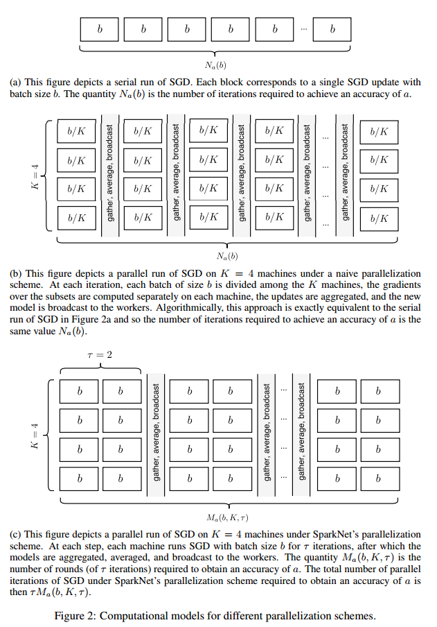


'MachineLearning' 카테고리의 다른 글
| SSD : Single Shot MultiBox Detector (0) | 2017.04.21 |
|---|---|
| YOLO CNN : Real-Time Object Detection (2) | 2017.04.12 |
| Machine Learning with the tools IPython Notebook SFrame (0) | 2017.02.05 |
| Machine Learning with the tools IPython Notebook Usage (0) | 2017.02.04 |
| Machine Learning with the tools IPython Notebook & GraphLab Create on AWS (0) | 2017.02.04 |