SSD : Single Shot MultiBox Detector
Reference
Wei Liu1, Dragomir Anguelov2, Dumitru Erhan3, Christian Szegedy3, Scott Reed4, Cheng-Yang Fu1, Alexander C. Berg1
1UNC Chapel Hill 2Zoox Inc. 3Google Inc. 4University of Michigan, Ann-Arbor 1wliu@cs.unc.edu, 2drago@zoox.com, 3{dumitru,szegedy}@google.com, 4reedscot@umich.edu, 1{cyfu,aberg}@cs.unc.edu
https://arxiv.org/abs/1512.02325
ABSTRACT
We present a method for detecting objects in images using a single deep neural network. Our approach, named SSD, discretizes the output space of bounding boxes into a set of default boxes over different aspect ratios and scales per feature map location. At prediction time, the network generates scores for the presence of each object category in each default box and produces adjustments to the box to better match the object shape. Additionally, the network combines predictions from multiple feature maps with different resolutions to naturally handle objects of various sizes. SSD is simple relative to methods that require object proposals because it completely eliminates proposal generation and subsequent pixel or feature resampling stages and encapsulates all computation in a single network. This makes SSD easy to train and straightforward to integrate into systems that require a detection component. Experimental results on the PASCAL VOC, COCO, and ILSVRC datasets confirm that SSD has competitive accuracy to methods that utilize an additional object proposal step and is much faster, while providing a unified framework for both training and inference. For 300 × 300 in- put, SSD achieves 74.3% mAP1 on VOC2007 test at 59 FPS on a Nvidia Titan X and for 512 × 512 input, SSD achieves 76.9% mAP, outperforming a comparable state-of-the-art Faster R-CNN model. Compared to other single stage methods, SSD has much better accuracy even with a smaller input image size. Code is available at: https://github.com/weiliu89/caffe/tree/ssd.
우리는 하나의 심층 신경망 (deep neural network)을 사용하여 이미지의 객체를 검출하는 방법을 제시합니다. SSD라는 이름의 접근 방식은 테두리 상자의 출력 공간을 기능 맵 위치별로 서로 다른 종횡비와 비율로 기본 상자 집합으로 이산합니다. 예측 시간에 네트워크는 각 기본 상자에서 각 개체 범주의 존재에 대한 점수를 생성하고, 개체 모양을 보다 잘 일치시키기 위해 상자를 조정합니다. 또한 네트워크는 다양한 해상도의 여러 기능 맵의 예측을 결합하여 다양한 크기의 개체를 자연스럽게 처리합니다. SSD는 제안서 생성 및 후속 픽셀 또는 기능 재 샘플링 단계를 완전히 제거하고 모든 계산을 단일 네트워크에 캡슐화하기 때문에 객체 제안을 필요로하는 방법에 비해 간단합니다. 이를 통해 SSD는 탐지 구성 요소가 필요한 시스템에 쉽게 통합 할 수 있습니다. PASCAL VOC, COCO 및 ILSVRC 데이터 세트에 대한 실험 결과에 따르면 SSD는 추가 객체 제안 단계를 사용하는 방법과 비교하여 정확성이 뛰어나며 교육(Training)과 추론(Inference) 모두에 통일된 프레임워크를 제공하면서 훨씬 빠릅니다. 300 × 300 입력의 경우 SSD는 Nvidia Titan X에서 59 FPS의 VOC 2007 테스트에서 74.3 % mAP1을 얻었고 512x512 입력의 경우 SSD는 76.9 % mAP를 달성하여 동급 최강의 빠른 R- CNN 모델. 다른 싱글 스테이지 방식에 비해 SSD는 입력 이미지 크기가 작을 때보 다 훨씬 더 정확합니다. 코드는 https://github.com/weiliu89/caffe/tree/ssd에서 사용할 수 있습니다.
Keywords : Real-time Object Detection; Convolutional Neural Network
1 Introduction
Current state-of-the-art object detection systems are variants of the following approach: hypothesize bounding boxes, resample pixels or features for each box, and apply a high- quality classifier. This pipeline has prevailed on detection benchmarks since the Selective Search work [1] through the current leading results on PASCAL VOC, COCO, and ILSVRC detection all based on Faster R-CNN[2] albeit with deeper features such as [3]. While accurate, these approaches have been too computationally intensive for embedded systems and, even with high-end hardware, too slow for real-time applications. Often detection speed for these approaches is measured in seconds per frame (SPF), and even the fastest high-accuracy detector, Faster R-CNN, operates at only 7 frames per second (FPS). There have been many attempts to build faster detectors by attacking each stage of the detection pipeline (see related work in Sec. 4), but so far, significantly increased speed comes only at the cost of significantly decreased detection accuracy.
현재의 최첨단 물체 감지 시스템은 다음과 같은 접근법의 변형입니다 : 경계 상자(bounding boxes)를 가정하고, 각 상자의 픽셀 또는 특징을 재 샘플링하고, 고품질 분류기를 적용합니다. 이 파이프 라인은 PASCAL VOC, COCO 및 ILSVRC 탐지의 최신 결과를 통해 Selective Search 작업 [1] 이후 탐지 벤치 마크에서 우세한 것으로, [3]과 같은 더 깊은 특징이 있음에도 불구하고 빠른 R-CNN을 기반으로합니다 [2]. 이러한 접근 방식은 정확하지만 임베디드 시스템에서는 너무 연산 집약적이었고 고급 하드웨어에서도 실시간 응용 프로그램에는 너무 느립니다. 이러한 접근 방식의 검출 속도는 프레임 당 초 단위 (SPF)로 측정되는 경우가 많으며 가장 빠른 고정밀 검출기 인 Faster R-CNN조차도 초당 7 프레임 (FPS)으로 작동합니다. 탐지 파이프 라인의 각 단계를 공격하여 더 빠른 탐지기를 구축하려는 시도가 많이 있었지만 (4 절의 관련 작업 참조) 지금까지는 감지(detection) 정확도(accuracy)가 현저히 떨어지는 대신 속도가 크게 향상되었습니다.
This paper presents the first deep network based object detector that does not resample pixels or features for bounding box hypotheses and and is as accurate as approaches that do. This results in a significant improvement in speed for high-accuracy detection (59 FPS with mAP 74.3% on VOC2007 test, vs. Faster R-CNN 7 FPS with mAP 73.2% or YOLO 45 FPS with mAP 63.4%). The fundamental improvement in speed comes from eliminating bounding box proposals and the subsequent pixel or feature resampling stage. We are not the first to do this (cf [4,5]), but by adding a series of improvements, we manage to increase the accuracy significantly over previous attempts. Our improvements include using a small convolutional filter to predict object categories and offsets in bounding box locations, using separate predictors (filters) for different aspect ratio detections, and applying these filters to multiple feature maps from the later stages of a network in order to perform detection at multiple scales. With these modifications—especially using multiple layers for prediction at different scales—we can achieve high-accuracy using relatively low resolution input, further increasing detection speed. While these contributions may seem small independently, we note that the resulting system improves accuracy on real-time detection for PASCAL VOC from 63.4% mAP for YOLO to 74.3% mAP for our SSD. This is a larger relative improvement in detection accuracy than that from the recent, very high-profile work on residual networks [3]. Furthermore, significantly improving the speed of high-quality detection can broaden the range of settings where computer vision is useful.
이 논문은 바운딩 박스 가설에 대해 픽셀이나 피쳐를 재 샘플링하지 않는 최초의 딥 네트워크 기반의 객체 검출기를 제시하며, 그러한 접근법만큼 정확합니다. 그 결과 고정밀도 검출 (VOP2007 테스트에서 mAP 74.3 %, mAP 73.2 %를 사용하는 Faster R-CNN 7 FPS 또는 mAP 63.4 %를 사용하는 YOLO 45 FPS)에 비해 속도가 크게 향상되었습니다. 속도의 근본적인 향상은 경계 상자 제안과 후속 픽셀 또는 특징(feature) 리샘플링 단계를 없앰으로써 가능합니다. 우리는 이것을 처음으로하는 것은 아니지만 (cf [4,5]) 일련의 개선 사항을 추가함으로써 이전 시도에 비해 정확성을 크게 높일 수 있습니다. 우리의 개선점으로는 작은 컨볼루션 필터를 사용하여 경계 상자 위치에서 객체 카테고리 및 오프셋을 예측하고, 다른 종횡비 감지에 대해 별도의 예측기(필터)를 사용하고, 네트워크의 후기 단계에서 이러한 필터를 적용하여 수행 할 수 있습니다 여러 척도에서의 탐지. 이러한 수정을 통해 (특히 여러 척도의 예측을 위해 여러 레이어 사용) 상대적으로 낮은 해상도의 입력을 사용하여 고정밀 도로 검색 속도를 높일 수 있습니다. 이러한 기여도는 독립적으로 보일 수 있지만, 결과 시스템은 PASCAL VOC의 실시간 탐지 정확도를 YOLO의 경우 63.4 %에서 SSD의 경우 74.3 %로 향상시킵니다. 이는 잔여 네트워크에 대한 최근의 매우 중요한 작업에서보다 탐지 정확도에서 더 큰 상대적인 향상이다 [3]. 또한 고품질 감지 속도를 크게 향상 시키면 컴퓨터 비전이 유용한 설정 범위를 넓힐 수 있습니다.
We summarize our contributions as follows:
We introduce SSD, a single-shot detector for multiple categories that is faster than the previous state-of-the-art for single shot detectors (YOLO), and significantly more accurate, in fact as accurate as slower techniques that perform explicit region proposals and pooling (including Faster R-CNN).
The core of SSD is predicting category scores and box offsets for a fixed set of default bounding boxes using small convolutional filters applied to feature maps. To achieve high detection accuracy we produce predictions of different scales from feature maps of different scales, and explicitly separate predictions by aspect ratio. These design features lead to simple end-to-end training and high accuracy, even on low resolution input images, further improving the speed vs accuracy trade-off. Experiments include timing and accuracy analysis on models with varying input size evaluated on PASCAL VOC, COCO, and ILSVRC and are compared to a range of recent state-of-the-art approaches.
우리는 우리의 공헌을 다음과 같이 요약합니다 :
우리는 싱글 샷 검출기(YOLO)에 대한 이전의 최첨단 기술보다 더 빠른 여러 범주의 단일 샷 검출기 인 SSD를 소개하고 명시 적 영역 제안을 수행하는 더 느린 기술만큼 정확하고 훨씬 정확합니다 및 풀링 (빠른 R-CNN 포함).
SSD의 핵심은 기능 맵에 적용된 작은 컨볼 루션 필터를 사용하여 고정 된 기본 경계 상자 집합에 대한 범주 점수 및 상자 오프셋을 예측하는 것입니다. 높은 탐지 정확도를 달성하기 위해 서로 다른 스케일의 기능 맵과 다른 스케일의 예측을 생성하고 명시 적으로 종횡비별로 예측을 분리합니다. 이러한 디자인 기능은 저해상도 입력 이미지 에서조차 간단한 엔드 투 엔드 (end-to-end) 교육과 높은 정확도를 제공하여 속도와 정확도의 균형을 더욱 향상시킵니다. 실험에는 PASCAL VOC, COCO 및 ILSVRC에서 평가되는 다양한 입력 크기를 가진 모델에 대한 타이밍 및 정확도 분석이 포함되며 최근의 최첨단 접근 방식과 비교됩니다.
2 The Single Shot Detector (SSD)
This section describes our proposed SSD framework for detection (Sec. 2.1) and the associated training methodology (Sec. 2.2). Afterwards, Sec. 3 presents dataset-specific model details and experimental results.
이 절에서는 제안 된 SSD 탐지 프레임 워크 (2.1 절)와 관련 교육 방법론 (2.2 절)에 대해 설명합니다. 그 후에, Sec. 3은 데이터 집합 별 모델 세부 정보 및 실험 결과를 나타냅니다.

Fig. 1: SSD framework. (a) SSD only needs an input image and ground truth boxes for each object during training. In a convolutional fashion, we evaluate a small set (e.g. 4) of default boxes of different aspect ratios at each location in several feature maps with different scales (e.g. 8 × 8 and 4 × 4 in (b) and (c)). For each default box, we predict both the shape offsets and the confidences for all object categories ((c1 , c2 , · · · , cp )). At training time, we first match these default boxes to the ground truth boxes. For example, we have matched two default boxes with the cat and one with the dog, which are treated as positives and the rest as negatives. The model loss is a weighted sum between localization loss (e.g. Smooth L1 [6]) and confidence loss (e.g. Softmax).
그림. 1 : SSD 프레임 워크. (a) SSD는 훈련 중 각 물체에 대한 입력 이미지 및 접지 진실 상자 만 필요합니다. 컨벌루션 방식으로, 우리는 다른 측면 여러 특징 맵의 각 위치에서 다른 화면 비율의 기본 상자의 작은 세트를 (예를 들어, 4) 평가 (예를 들어, 8 × 8, 4 × 4 (b)와 (c)). 각 기본 상자, 우리는 모양 오프셋 및 모든 개체 종류에 대한 비밀도 ((C1, C2, · · ·, CP))를 모두 예측하고있다. 교육 시간에, 우리는 먼저이 기본 상자를 지상 진실 상자와 일치시킵니다. 예를 들어, 우리는 긍정과 부정과 나머지로 취급되는 두 개의 기본 고양이와 상자와 개를, 일치했다. 모델 손실 파악 손실 (예를 들어 부드러운 L1 [6])와 지수 손실 (예를 들어, 소프트 맥스) 사이의 가중된 합이다.
2.1 Model
The SSD approach is based on a feed-forward convolutional network that produces a fixed-size collection of bounding boxes and scores for the presence of object class instances in those boxes, followed by a non-maximum suppression step to produce the final detections. The early network layers are based on a standard architecture used for high quality image classification (truncated before any classification layers), which we will call the base network2. We then add auxiliary structure to the network to produce detections with the following key features:
SSD 접근 방식은 고정 박스 크기의 경계 상자 모음과 해당 상자에있는 개체 클래스 인스턴스의 존재 여부에 대한 점수를 생성하는 피드 포워드 컨볼 루션 네트워크를 기반으로하며 최종 탐지를 생성하는 비 최대 억제 단계가 뒤 따른다. 초기 네트워크 계층은 고품질 이미지 분류 (모든 분류 계층 전에 절단 됨)에 사용되는 표준 아키텍처를 기반으로하며이를 기본 네트워크 2라고합니다. 그런 다음 네트워크에 보조 구조를 추가하여 다음과 같은 주요 기능을 갖춘 탐지를 생성합니다.
Multi-scale feature maps for detection We add convolutional feature layers to the end of the truncated base network. These layers decrease in size progressively and allow predictions of detections at multiple scales. The convolutional model for predicting detections is different for each feature layer (cf Overfeat[4] and YOLO[5] that operate on a single scale feature map).
탐지를 위한 다중 스케일 피쳐 맵 절단 된 기본 네트워크의 끝에 컨볼 루션 피쳐 레이어를 추가합니다. 이러한 레이어는 점진적으로 크기가 감소하고 여러 배율에서 감지를 예측할 수 있습니다. 탐지를 예측하기위한 컨볼 루션 모델은 각 기능 레이어마다 다릅니다 (단일 배율 피쳐 맵에서 작동하는 Overfeat [4] 및 YOLO [5] 참조).
Convolutional predictors for detection Each added feature layer (or optionally an existing feature layer from the base network) can produce a fixed set of detection predictions using a set of convolutional filters. These are indicated on top of the SSD network architecture in Fig. 2. For a feature layer of size m × n with p channels, the basic element for predicting parameters of a potential detection is a 3 × 3 × p small kernel that produces either a score for a category, or a shape offset relative to the default box coordinates. At each of the m × n locations where the kernel is applied, it produces an output value. The bounding box offset output values are measured relative to a default box position relative to each feature map location (cf the architecture of YOLO[5] that uses an intermediate fully connected layer instead of a convolutional filter for this step).
탐지를위한 컨벌루션 예측자 추가된 각 피쳐 레이어 (또는 선택적으로 기본 네트워크의 기존 피쳐 레이어)는 컨벌루션 필터 세트를 사용하여 고정 된 탐지 예측 세트를 생성 할 수 있습니다. 이는 그림 1의 SSD 네트워크 아키텍처의 상단에 표시됩니다. 2. p 채널을 갖는 크기 m × n의 Feature 레이어의 경우, 잠재적 인 검출의 매개 변수를 예측하기위한 기본 요소는 범주에 대한 점수를 산출하는 3x3xp의 작은 커널 또는 기본 상자 좌표. 커널이 적용되는 mxn 위치 각각에서 출력 값을 생성합니다. 바운딩 박스 오프셋 출력 값은 각 Feature 맵 위치와 관련된 기본 상자 위치에 상대적으로 측정됩니다 (이 단계에서 컨벌루션 필터 대신 중간 완전 연결 레이어를 사용하는 YOLO [5] 아키텍처 참조).

Fig. 2: A comparison between two single shot detection models: SSD and YOLO [5]. Our SSD model adds several feature layers to the end of a base network, which predict the offsets to default boxes of different scales and aspect ratios and their associated confidences. SSD with a 300 × 300 input size significantly outperforms its 448 × 448 YOLO counterpart in accuracy on VOC2007 test while also improving the speed.
그림. 2 : 두 개의 단일 샷 검출 모델 인 SSD와 YOLO [5]의 비교. 우리의 SSD 모델은 기본 네트워크의 끝 부분에 몇 가지 기능 레이어를 추가합니다.이 기능 레이어는 서로 다른 크기와 종횡비 및 관련 신뢰도의 기본 상자에 대한 오프셋을 예측합니다. 300 × 300 입력 크기의 SSD는 VOC2007 테스트의 정확도에서 448 × 448 YOLO 성능보다 월등히 뛰어남과 동시에 속도가 향상되었습니다.
Default boxes and aspect ratios We associate a set of default bounding boxes with each feature map cell, for multiple feature maps at the top of the network. The default boxes tile the feature map in a convolutional manner, so that the position of each box relative to its corresponding cell is fixed. At each feature map cell, we predict the offsets relative to the default box shapes in the cell, as well as the per-class scores that indicate the presence of a class instance in each of those boxes. Specifically, for each box out of k at a given location, we compute c class scores and the 4 offsets relative to the original default box shape. This results in a total of (c + 4)k filters that are applied around each location in the feature map, yielding (c + 4)kmn outputs for a m × n feature map. For an illustration of default boxes, please refer to Fig. 1. Our default boxes are similar to the anchor boxes used in Faster R-CNN [2], however we apply them to several feature maps of different resolutions. Allowing different default box shapes in several feature maps let us efficiently discretize the space of possible output box shapes.
기본 상자 및 가로 세로 비율 기본 테두리 상자 세트를 각 기능 맵 셀과 연결하여 네트워크 맨 위에있는 여러 기능 맵을 찾습니다. 기본 상자는 기능 맵을 컨볼 루션 방식으로 배열하여 각 상자의 해당 셀에 대한 위치가 고정되도록합니다. 각 피쳐 지도 셀에서 셀의 기본 상자 모양과 관련된 오프셋과 각 상자에 클래스 인스턴스가 있음을 나타내는 클래스 별 점수를 예측합니다. 특히 주어진 위치에서 k의 각 상자에 대해 원래의 기본 상자 모양과 관련하여 c 클래스 점수와 4 개의 오프셋을 계산합니다. 그 결과, (c + 4) k 개의 필터가 기능 맵의 각 위치 주변에 적용되어 m × n 피쳐 맵에 대해 (c + 4) kmn 출력을 산출합니다. 기본 상자에 대한 설명은 그림 2를 참조하십시오. 1. 우리의 기본 박스는 Faster R-CNN [2]에서 사용 된 앵커 박스와 비슷하지만 해상도가 다른 여러 개의 기능 맵에 적용합니다. 여러 가지 기능 맵에서 다른 기본 상자 모양을 허용하면 가능한 출력 상자 모양의 공간을 효율적으로 분리 할 수 있습니다.
2.2 Training
The key difference between training SSD and training a typical detector that uses region proposals, is that ground truth information needs to be assigned to specific outputs in the fixed set of detector outputs. Some version of this is also required for training in YOLO[5] and for the region proposal stage of Faster R-CNN[2] and MultiBox[7]. Once this assignment is determined, the loss function and backpropagation are applied end- to-end. Training also involves choosing the set of default boxes and scales for detection as well as the hard negative mining and data augmentation strategies.
SSD 교육과 지역 제안서를 사용하는 일반적인 탐지기 교육의 주요 차이점은 지상 진실 정보를 고정 된 감지기 출력 세트의 특정 출력에 할당해야한다는 것입니다. 이 중 일부 버전은 YOLO [5]의 교육 및 Faster R-CNN [2] 및 MultiBox [7]의 지역 제안 단계에도 필요합니다. 일단이 할당이 결정되면, 손실 함수 및 역 전파가 종단 간 적용됩니다. 또한 교육에는 하드 네거티브 마이닝 및 데이터 확대 전략뿐 아니라 탐지 용 기본 상자 및 눈금 세트 선택이 포함됩니다.
Matching strategy During training we need to determine which default boxes correspond to a ground truth detection and train the network accordingly. For each ground truth box we are selecting from default boxes that vary over location, aspect ratio, and scale. We begin by matching each ground truth box to the default box with the best jaccard overlap (as in MultiBox [7]). Unlike MultiBox, we then match default boxes to any ground truth with jaccard overlap higher than a threshold (0.5). This simplifies the learning problem, allowing the network to predict high scores for multiple overlapping default boxes rather than requiring it to pick only the one with maximum overlap.
일치하는 전략 훈련 중 우리는 지상실 진위 감지에 해당하는 기본 상자를 판별하고 이에 따라 네트워크를 훈련해야합니다. 각 지상 진실 상자에 대해 우리는 위치, 종횡비 및 규모에 따라 다른 기본 상자에서 선택합니다. 우선 각 진실 상자를 가장 좋은 jaccard가 겹치는 기본 상자에 일치 시켜서 시작합니다 (MultiBox [7] 에서처럼). MultiBox와는 달리 임계 값 (0.5)보다 높은 jaccard 겹침을 사용하여 기본 상자를 접지 진리와 일치시킵니다. 이것은 학습 문제를 단순화하여, 네트워크가 최대 겹침이있는 것을 선택하도록 요구하지 않고, 다수의 겹쳐진 디폴트 박스에 대한 높은 점수를 예측할 수있게한다.
Training objective The SSD training objective is derived from the MultiBox objective[7,8]but is extended to handle multiple object categories. Let xpij ={1,0} be an indicator for matching the i-th default box to the j-th ground truth box of category p. In the matching strategy above, we can have i xpij ≥ 1. The overall objective loss function is a weighted sum of the localization loss (loc) and the confidence loss (conf):
교육 목표 SSD 교육 목표는 MultiBox 목표 [7,8]에서 파생되었지만 여러 객체 카테고리를 처리하도록 확장되었습니다. xpij = {1,0}을 i 번째 기본 상자를 범주 p의 j 번째 접지 상자에 일치시키는 지표로 둡니다. 위의 매칭 전략에서, 우리는 i xpij ≥ 1을 가질 수있다. 전반적인 목표 손실 함수는 위치 파악 손실 (loc)과 신뢰 손실 (conf)의 가중치 합이다.

where N is the number of matched default boxes. If N = 0, wet set the loss to 0. The localization loss is a Smooth L1 loss [6] between the predicted box (l) and the ground truth box (g) parameters. Similar to Faster R-CNN [2], we regress to offsets for the center (cx, cy) of the default bounding box (d) and for its width (w) and height (h).
여기서 N은 일치하는 기본 상자의 수입니다. N = 0이면 손실을 0으로 설정합니다. 위치 파악 손실은 예측 상자 (l)와 접지 실 상자 (g) 매개 변수 사이의 부드러운 L1 손실입니다 [6]. Faster R-CNN [2]과 마찬가지로 기본 경계 상자 (d)의 중심 (cx, cy)과 폭 (w) 및 높이 (h)에 대한 오프셋으로 회귀합니다.

The confidence loss is the softmax loss over multiple classes confidences (c).
신뢰 손실은 여러 클래스 신뢰도 (c)에 대한 softmax 손실입니다.

and the weight term α is set to 1 by cross validation.
교차 검증에 의해 가중 항 α가 1로 설정된다.
Choosing scales and aspect ratios for default boxes To handle different object scales, some methods [4,9] suggest processing the image at different sizes and combining the results afterwards. However, by utilizing feature maps from several different layers in a single network for prediction we can mimic the same effect, while also sharing parameters across all object scales. Previous works [10,11] have shown that using feature maps from the lower layers can improve semantic segmentation quality because the lower layers capture more fine details of the input objects. Similarly, [12] showed that adding global context pooled from a feature map can help smooth the segmentation results. Motivated by these methods, we use both the lower and upper feature maps for detection. Figure 1 shows two exemplar feature maps (8 × 8 and 4 × 4) which are used in the framework. In practice, we can use many more with small computational overhead.
기본 상자의 비율 및 종횡비 선택 서로 다른 객체 크기를 처리하기 위해 일부 방법 [4,9]에서는 이미지를 다른 크기로 처리하고 나중에 결과를 결합하는 것이 좋습니다. 그러나 예측을 위해 단일 네트워크에서 여러 레이어의 기능 맵을 활용함으로써 동일한 효과를 모방하고 모든 객체 척도에서 매개 변수를 공유 할 수 있습니다. 이전 연구 [10,11]에서는 하위 계층이 입력 객체의 세부 묘사를 더 잘 포착하기 때문에 하위 계층의 특성 맵을 사용하면 의미론적 세분화 품질을 향상시킬 수 있다는 것을 보여주었습니다. 유사하게, [12]는 feature map으로부터 풀링 된 global context를 추가하는 것이 segmentation 결과를 부드럽게하는데 도움을 줄 수 있음을 보였다. 이 방법들에 의해 동기 부여를 위해 우리는 탐지를 위해 하부 및 상부 특징 맵 모두를 사용한다. 그림 1은 프레임 워크에서 사용되는 두 개의 표본 피쳐 맵 (8 × 8 및 4 × 4)을 보여줍니다. 실제로는 적은 계산 오버 헤드로 더 많은 것을 사용할 수 있습니다.
Feature maps from different levels within a network are known to have different (empirical) receptive field sizes [13]. Fortunately, within the SSD framework, the de- fault boxes do not necessary need to correspond to the actual receptive fields of each layer. We design the tiling of default boxes so that specific feature maps learn to be responsive to particular scales of the objects. Suppose we want to use m feature maps for prediction. The scale of the default boxes for each feature map is computed as:
네트워크 내의 서로 다른 레벨의 특성 맵은 서로 다른 (경험적) 수용 필드 크기를 갖는 것으로 알려져있다 [13]. 다행스럽게도 SSD 프레임 워크 내에서 기본 상자는 각 계층의 실제 수용 필드와 일치 할 필요는 없습니다. 특정 기능 맵이 객체의 특정 축척에 반응하는 것을 배우도록 기본 상자의 기와(tiling)를 디자인합니다. 예측을 위해 m 개의 피처 맵을 사용한다고 가정합니다. 각 기능 맵의 기본 상자 크기는 다음과 같이 계산됩니다.

where smin is 0.2 and smax is 0.9, meaning the lowest layer has a scale of 0.2 and the highest layer has a scale of 0.9, and all layers in between are regularly spaced. We impose different aspect ratios for the default boxes, and denote them as ar ∈ {1, 2, 3, 1 2 , 1 3 }. We can compute the width (w a k = sk √ ar) and height (h a k = sk/ √ ar) for each default box. For the aspect ratio of 1, we also add a default box whose scale is s 0 k = √sksk+1, resulting in 6 default boxes per feature map location. We set the center of each default box to ( i+0.5 |fk| , j+0.5 |fk| ), where |fk| is the size of the k-th square feature map, i, j ∈ [0, |fk|). In practice, one can also design a distribution of default boxes to best fit a specific dataset. How to design the optimal tiling is an open question as well.
smin이 0.2이고 smax가 0.9 인 경우 가장 낮은 레이어는 0.2의 눈금을 가지며 가장 높은 레이어는 0.9의 눈금을 가지며 그 사이의 모든 레이어는 규칙적으로 간격을두고 있습니다. 우리는 디폴트 박스들에 대해 다른 종횡비를 부과하고 그것들을 ar ∈ {1, 2, 3, 1 2, 1 3}로 표시한다. 각 기본 상자의 너비 (w a k = sk √ ar)와 높이 (h a k = sk / √ ar)를 계산할 수 있습니다. 종횡비가 1 인 경우 축척이 s 0 k = √ sksk + 1 인 기본 상자를 추가하여 피쳐지도 위치 당 6 개의 기본 상자가 생성됩니다. 각 기본 상자의 중심을 (i + 0.5 | fk |, j + 0.5 | fk |)로 설정합니다. 여기서 | fk | 는 k 번째 사각형 특징 맵의 크기, i, j ∈ [0, | fk |)이다. 실제로는 특정 데이터 세트에 가장 잘 맞는 기본 상자를 디자인 할 수도 있습니다. 최적의 타일링을 설계하는 방법도 공개적인 질문입니다.
By combining predictions for all default boxes with different scales and aspect ratios from all locations of many feature maps, we have a diverse set of predictions, covering various input object sizes and shapes. For example, in Fig. 1, the dog is matched to a default box in the 4 × 4 feature map, but not to any default boxes in the 8 × 8 feature map. This is because those boxes have different scales and do not match the dog box, and therefore are considered as negatives during training.
모든 기본 기능 상자에 대한 예측을 여러 기능 맵의 모든 위치에서 다른 비율 및 종횡비로 결합하여 다양한 입력 개체 크기 및 모양을 포괄하는 다양한 예측을 제공합니다. 예를 들어, Fig. 1이면 개가 4x4 기능 맵에서 기본 상자와 일치하지만 8x8 기능 맵에서는 기본 상자와 일치하지 않습니다. 이러한 상자는 다른 크기와 도그 박스와 일치하지 않기 때문에 훈련 중에 네거티브로 간주되기 때문입니다.
Hard negative mining After the matching step, most of the default boxes are negatives, especially when the number of possible default boxes is large. This introduces a significant imbalance between the positive and negative training examples. Instead of using all the negative examples, we sort them using the highest confidence loss for each default box and pick the top ones so that the ratio between the negatives and positives is at most 3:1. We found that this leads to faster optimization and a more stable training.
단점 마이닝 (Hard Negative mining) 매칭 단계가 끝나면 기본 상자의 대부분이 네거티브이며, 특히 가능한 기본 상자 수가 많으면 특히 그렇습니다. 이것은 긍정적 인 것과 부정적인 훈련의 예들 사이에 상당한 불균형을 가져온다. 모든 음화 예제를 사용하는 대신, 각 기본 상자에 대해 가장 높은 신뢰도 손실을 사용하여 정렬하고 음수와 양수 비율이 3 : 1 이하가되도록 상위 상자를 선택합니다. 우리는 이것이보다 빠른 최적화와보다 안정적인 교육을 유도한다는 것을 발견했습니다.
Data augmentation To make the model more robust to various input object sizes and shapes, each training image is randomly sampled by one of the following options:
데이터 증가 다양한 입력 개체 크기 및 모양에 대한 모델을보다 강력하게 만들기 위해 각 교육 이미지는 다음 옵션 중 하나에 의해 무작위로 샘플링됩니다.
– Use the entire original input image.
– Sample a patch so that the minimum jaccard overlap with the objects is 0.1, 0.3, 0.5, 0.7, or 0.9.
- Randomly sample a patch.
- 원본 입력 이미지 전체를 사용하십시오.
- 최소 jaccard가 오브젝트와 겹치도록 패치를 샘플링하여 0.1, 0.3, 0.5, 0.7 또는 0.9가되도록하십시오.
- 무작위로 패치를 샘플링하십시오.
The size of each sampled patch is [0.1, 1] of the original image size, and the aspect ratio is between 1 2 and 2. We keep the overlapped part of the ground truth box if the center of it is in the sampled patch. After the aforementioned sampling step, each sampled patch is resized to fixed size and is horizontally flipped with probability of 0.5, in addition to applying some photo-metric distortions similar to those described in [14].
샘플링 된 각 패치의 크기는 원본 이미지 크기의 [0.1, 1]이고 종횡비는 1 2 2입니다. 중심이 샘플링 된 패치에있는 경우 지상 진실 상자의 중첩 된 부분을 유지합니다. 앞서 언급 한 샘플링 단계 후에 샘플링 된 각 패치는 고정 크기로 크기가 조정되고 [14]에서 설명한 것과 유사한 몇 가지 사진 메트릭 왜곡을 적용 할뿐만 아니라 0.5의 확률로 수평으로 대칭 이동됩니다.
3 Experimental Results
Base network Our experiments are all based on VGG16 [15], which is pre-trained on the ILSVRC CLS-LOC dataset [16]. Similar to DeepLab-LargeFOV [17], we convert fc6 and fc7 to convolutional layers, subsample parameters from fc6 and fc7, change pool5 from 2 × 2 − s2 to 3 × 3 − s1, and use the a trous ` algorithm [18] to fill the ”holes”. We remove all the dropout layers and the fc8 layer. We fine-tune the resulting model using SGD with initial learning rate 10−3 , 0.9 momentum, 0.0005 weight decay, and batch size 32. The learning rate decay policy is slightly different for each dataset, and we will describe details later. The full training and testing code is built on Caffe [19] and is open source at: https://github.com/weiliu89/caffe/tree/ssd.
기본 네트워크 우리의 실험은 모두 ILSVRC CLS-LOC 데이터 세트 [16]에 사전 교육 된 VGG16 [15]을 기반으로합니다. DeepLab-LargeFOV [17]와 마찬가지로, fc6와 fc7을 convolutional layer로 변환하고, fc6와 fc7의 서브 샘플 파라미터를 2x2 - s2에서 3x3 - s1로 변경하고, trous 알고리즘 [18] "구멍"을 채우기 위해. 우리는 모든 드롭 아웃 레이어와 fc8 레이어를 제거합니다. SGD를 사용하여 결과 모델을 초기 학습 속도 10-3, 0.9 운동량, 0.0005 무게 감소 및 배치 크기 32로 미세 조정합니다. 학습 속도 감소 정책은 각 데이터 세트마다 약간 씩 다르며 나중에 자세히 설명 할 것입니다. 전체 교육 및 테스트 코드는 Caffe [19]를 기반으로하며 https://github.com/weiliu89/caffe/tree/ssd에서 공개 소스입니다.
3.1 PASCAL VOC2007
On this dataset, we compare against Fast R-CNN [6] and Faster R-CNN [2] on VOC2007 test (4952 images). All methods fine-tune on the same pre-trained VGG16 network.
이 데이터 세트에서 VOC2007 테스트 (4952 개 이미지)에서 Fast R-CNN [6]과 Faster R-CNN [2]을 비교합니다. 모든 방법은 동일한 사전 훈련 된 VGG16 네트워크를 미세 조정합니다.
Figure 2 shows the architecture details of the SSD300 model. We use conv4 3, conv7 (fc7), conv8 2, conv9 2, conv10 2, and conv11 2 to predict both location and confidences. We set default box with scale 0.1 on conv4 3 3 . We initialize the parameters for all the newly added convolutional layers with the ”xavier” method [20]. For conv4 3, conv10 2 and conv11 2, we only associate 4 default boxes at each feature map location – omitting aspect ratios of 1 3 and 3. For all other layers, we put 6 default boxes as described in Sec. 2.2. Since, as pointed out in [12], conv4 3 has a different feature scale compared to the other layers, we use the L2 normalization technique introduced in [12] to scale the feature norm at each location in the feature map to 20 and learn the scale during back propagation. We use the 10−3 learning rate for 40k iterations, then continue training for 10k iterations with 10−4 and 10−5 . When training on VOC2007 trainval, Table 1 shows that our low resolution SSD300 model is already more accurate than Fast R-CNN. When we train SSD on a larger 512 × 512 input image, it is even more accurate, surpassing Faster R-CNN by 1.7% mAP. If we train SSD with more (i.e. 07+12) data, we see that SSD300 is already better than Faster R-CNN by 1.1% and that SSD512 is 3.6% better. If we take models trained on COCO trainval35k as described in Sec. 3.4 and fine-tuning them on the 07+12 dataset with SSD512, we achieve the best results: 81.6% mAP
그림 2는 SSD300 모델의 아키텍처 세부 정보를 보여줍니다. conv4 3, conv7 (fc7), conv8 2, conv9 2, conv10 2 및 conv11 2를 사용하여 위치와 신뢰도를 모두 예측합니다. conv4 3의 scale 0.1로 default box를 설정합니다. 3 3. "xavier"방법 [20]을 사용하여 새로 추가 된 모든 컨볼 루션 계층에 대한 매개 변수를 초기화합니다. conv4 3, conv10 2 및 conv11 2의 경우, 각 기능 맵 위치에 4 개의 기본 상자 만 연결합니다. 1-3 및 3의 종횡비는 생략합니다. 다른 모든 레이어의 경우 6 단계에서 설명한대로 6 개의 기본 상자를 넣습니다. 2.2. [12]에서 지적했듯이, conv4 3은 다른 계층에 비해 다른 특징 규모를 가지고 있기 때문에, [12]에서 소개 된 L2 정규화 기법을 사용하여 feature map의 각 위치에서의 feature norm을 20으로 스케일링하고 역 전파 중에 규모. 우리는 40-3 번의 반복에 대해 10-3 학습률을 사용하고 10-4 및 10-5로 10k 반복에 대한 학습을 계속합니다. VOC2007 trainval을 교육 할 때, 표 1은 우리의 저해상도 SSD300 모델이 이미 Fast R-CNN보다 더 정확하다는 것을 보여줍니다. 더 큰 512 × 512 입력 이미지에서 SSD를 학습 할 때, 훨씬 더 정확하여 빠른 R-CNN을 1.7 % mAP 능가합니다. 더 많은 (즉, 07 + 12) 데이터로 SSD를 교육하면 SSD300이 이미 Faster R-CNN보다 1.1 % 더 좋고 SSD512가 3.6 % 더 우수하다는 것을 알 수 있습니다. 우리가 COCO trainval 35k에서 훈련 된 모델을 Sec. 3.4와 SSD512로 07 + 12 데이터 세트에서 미세 조정하면 최상의 결과를 얻을 수 있습니다 : 81.6 % mAP.
To understand the performance of our two SSD models in more details, we used the detection analysis tool from [21]. Figure 3 shows that SSD can detect various object categories with high quality (large white area). The majority of its confident detections are correct. The recall is around 85-90%, and is much higher with “weak” (0.1 jaccard overlap) criteria. Compared to R-CNN [22], SSD has less localization error, indicating that SSD can localize objects better because it directly learns to regress the object shape and classify object categories instead of using two decoupled steps. However, SSD has more confusions with similar object categories (especially for animals), partly because we share locations for multiple categories. Figure 4 shows that SSD is very sensitive to the bounding box size. In other words, it has much worse performance on smaller objects than bigger objects. This is not surprising because those small objects may not even have any information at the very top layers. Increasing the input size (e.g. from 300×300 to 512×512) can help improve detecting small objects, but there is still a lot of room to improve. On the positive side, we can clearly see that SSD performs really well on large objects. And it is very robust to different object aspect ratios because we use default boxes of various aspect ratios per feature map location.
두 개의 SSD 모델의 성능을보다 자세히 이해하기 위해 [21]의 탐지 분석 도구를 사용했습니다. 그림 3은 SSD가 고품질 (큰 흰색 영역)의 다양한 객체 카테고리를 탐지 할 수 있음을 보여줍니다. 자체 탐지의 대부분은 정확합니다. 리콜은 약 85-90 %이며 "약한"(0.1 jaccard overlap) 기준으로 훨씬 높습니다. R-CNN [22]과 비교할 때 SSD는 지역화 오류가 적기 때문에 SSD는 두 개의 분리 된 단계를 사용하는 대신 객체 모양을 회귀하고 객체 범주를 직접 배울 수 있기 때문에 객체를 더 잘 지역화 할 수 있습니다. 그러나 SSD는 유사한 객체 카테고리 (특히 동물)와 더 많은 혼란을 빚고 있습니다. 부분적으로는 여러 카테고리에 대한 위치를 공유하기 때문입니다. 그림 4는 SSD가 테두리 상자 크기에 매우 민감하다는 것을 보여줍니다. 즉, 더 작은 물체는 큰 물체보다 훨씬 더 나쁜 성능을 보입니다. 이러한 작은 오브젝트는 맨 위의 레이어에 정보가 없기 때문에 놀라운 것은 아닙니다. 입력 크기를 늘리면 (예 : 300 × 300에서 512 × 512로) 작은 물체를 감지하는 데 도움이 될 수 있지만 개선해야 할 부분이 많이 남아 있습니다. 긍정적 인 측면에서 볼 때 SSD가 큰 개체에서 실제로 잘 수행되는지 확인할 수 있습니다. 또한 기능 맵 위치마다 다양한 종횡비의 기본 상자를 사용하기 때문에 다양한 오브젝트 종횡비에 매우 강력합니다.
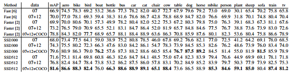
Table 1: PASCAL VOC2007 test detection results. Both Fast and Faster R-CNN use input images whose minimum dimension is 600. The two SSD models have exactly the same settings except that they have different input sizes (300×300 vs. 512×512). It is obvious that larger input size leads to better results, and more data always helps. Data: ”07”: VOC2007 trainval, ”07+12”: union of VOC2007 and VOC2012 trainval. ”07+12+COCO”: first train on COCO trainval35k then fine-tune on 07+12.
표 1 : PASCAL VOC2007 테스트 감지 결과. 빠른 속도와 빠른 R-CNN은 최소 치수가 600 인 입력 이미지를 사용합니다. 두 SSD 모델은 입력 크기가 서로 다른 것을 제외하고는 정확히 동일한 설정을 사용합니다 (300 × 300 대 512 × 512). 입력 크기가 커지면 결과가 더 좋아지고 데이터가 많을수록 항상 도움이됩니다. 데이터 : "07": VOC2007 trainval, "07 + 12": VOC2007 및 VOC2012 trainval의 조합. "07 + 12 + COCO": 첫 번째 열차는 COCO trainval35k에서 07 + 12에서 미세 조정합니다.
3.2 Model analysis
To understand SSD better, we carried out controlled experiments to examine how each component affects performance. For all the experiments, we use the same settings and input size (300 × 300), except for specified changes to the settings or component(s).
SSD를 더 잘 이해하기 위해 제어 된 실험을 수행하여 각 구성 요소가 성능에 어떤 영향을 주는지 조사했습니다. 모든 실험에서 설정이나 구성 요소에 지정된 변경 사항을 제외하고 동일한 설정과 입력 크기 (300 × 300)를 사용합니다.

Table 2: Effects of various design choices and components on SSD performance.
표 2 : SSD 성능에 대한 다양한 설계 선택 및 구성 요소의 영향.
Data augmentation is crucial. Fast and Faster R-CNN use the original image and the horizontal flip to train. We use a more extensive sampling strategy, similar to YOLO [5]. Table 2 shows that we can improve 8.8% mAP with this sampling strategy. We do not know how much our sampling strategy will benefit Fast and Faster R-CNN, but they are likely to benefit less because they use a feature pooling step during classification that is relatively robust to object translation by design.
데이터 증가가 중요합니다. 빠르고 빠른 R-CNN은 원본 이미지와 수평 플립을 사용하여 훈련합니다. 우리는 YOLO [5]와 비슷한보다 광범위한 샘플링 전략을 사용합니다. 표 2는이 샘플링 전략으로 8.8 % mAP를 개선 할 수 있음을 보여줍니다. 우리는 샘플링 전략이 Fast and Faster R-CNN에 얼마나 도움이되는지 알지 못하지만 분류 과정에서 객체 풀이에 상대적으로 견고한 기능 풀링 단계를 사용하기 때문에 이점이 적습니다.

Fig. 3: Visualization of performance for SSD512 on animals, vehicles, and furniture from VOC2007 test. The top row shows the cumulative fraction of detections that are correct (Cor) or false positive due to poor localization (Loc), confusion with similar categories (Sim), with others (Oth), or with background (BG). The solid red line reflects the change of recall with strong criteria (0.5 jaccard overlap) as the number of detections increases. The dashed red line is using the weak criteria (0.1 jaccard overlap). The bottom row shows the distribution of top-ranked false positive types.
그림 3 : VOC2007 테스트에서 동물, 차량 및 가구에 대한 SSD512의 성능 시각화. 맨 위 행에는 현지화가 좋지 않아 (Loc), 비슷한 카테고리와 혼동 (Sim), 다른 사람 (Oth) 또는 배경 (BG)으로 인해 올바른 (Cor) 또는 잘못된 양성인 탐지 누적 수가 표시됩니다. 적색 선은 검출 횟수가 증가함에 따라 강력한 기준 (0.5 초 카드 겹침)으로 리콜 변경을 반영합니다. 점선 빨간색 선은 약한 기준 (0.1 jaccard overlap)을 사용합니다. 맨 아래 행은 위 순위가 잘못된 유형의 분포를 보여줍니다.
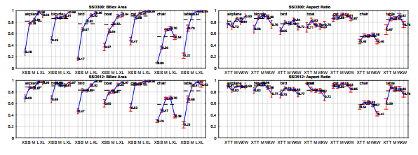
Fig. 4: Sensitivity and impact of different object characteristics on VOC2007 test set using [21]. The plot on the left shows the effects of BBox Area per category, and the right plot shows the effect of Aspect Ratio. Key: BBox Area: XS=extra-small; S=small; M=medium; L=large; XL =extra-large. Aspect Ratio: XT=extra-tall/narrow; T=tall; M=medium; W=wide; XW =extra-wide.
그림. 4 : [21]을 사용하여 VOC2007 테스트 세트에서 다른 물체 특성의 감도 및 영향. 왼쪽 그림은 카테고리 당 BBox Area의 효과를 보여주고 오른쪽 그림은 종횡비의 효과를 보여줍니다. 키 : BBox 면적 : XS = extra-small; S = 작음; M = 중간; L = 큰; XL = 초대형. 종횡비 : XT = extra-tall / narrow; T = 신장; M = 중간; W = 와이드; XW = 엑스트라 와이드.
More default box shapes is better. As described in Sec. 2.2, by default we use 6 default boxes per location. If we remove the boxes with 1 3 and 3 aspect ratios, the performance drops by 0.6%. By further removing the boxes with 1 2 and 2 aspect ratios, the performance drops another 2.1%. Using a variety of default box shapes seems to make the task of predicting boxes easier for the network.
더 많은 기본 상자 모양이 좋습니다. Sec. 2.2에서는 기본적으로 위치 당 6 개의 기본 상자를 사용합니다. 1 3 및 3 종횡비의 상자를 제거하면 성능이 0.6 % 떨어집니다. 1 2 및 2 종횡비의 상자를 추가로 제거하면 성능이 2.1 % 더 떨어집니다. 다양한 기본 상자 모양을 사용하면 네트워크를 쉽게 예측할 수 있습니다.
Atrous is faster. As described in Sec. 3, we used the atrous version of a subsampled VGG16, following DeepLab-LargeFOV [17]. If we use the full VGG16, keeping pool5 with 2 × 2 − s2 and not subsampling parameters from fc6 and fc7, and add conv5 3 for prediction, the result is about the same while the speed is about 20% slower.
Atrous가 빠릅니다. Sec. 3, 우리는 DeepLab-LargeFOV [17]에 따라 서브 샘플링 된 VGG16의 atrous 버전을 사용했습니다. 전체 VGG16을 사용하고 pool5를 2x2 - s2로 유지하고 fc6 및 fc7에서 서브 샘플링 매개 변수가 아니라 예측을 위해 conv5 3을 더하면 결과는 거의 동일하지만 속도는 약 20 % 느립니다.

Table 3: Effects of using multiple output layers.
표 3 : 다중 출력 레이어 사용의 효과.
Multiple output layers at different resolutions is better. A major contribution of SSD is using default boxes of different scales on different output layers. To measure the advantage gained, we progressively remove layers and compare results. For a fair comparison, every time we remove a layer, we adjust the default box tiling to keep the total number of boxes similar to the original (8732). This is done by stacking more scales of boxes on remaining layers and adjusting scales of boxes if needed. We do not exhaustively optimize the tiling for each setting. Table 3 shows a decrease in accuracy with fewer layers, dropping monotonically from 74.3 to 62.4. When we stack boxes of multiple scales on a layer, many are on the image boundary and need to be handled carefully. We tried the strategy used in Faster R-CNN [2], ignoring boxes which are on the boundary. We observe some interesting trends. For example, it hurts the performance by a large margin if we use very coarse feature maps (e.g. conv11 2 (1 × 1) or conv10 2 (3 × 3)). The reason might be that we do not have enough large boxes to cover large objects after the pruning. When we use primarily finer resolution maps, the performance starts increasing again because even after pruning a sufficient number of large boxes remains. If we only use conv7 for prediction, the performance is the worst, reinforcing the message that it is critical to spread boxes of different scales over different layers. Besides, since our predictions do not rely on ROI pooling as in [6], we do not have the collapsing bins problem in low-resolution feature maps [23]. The SSD architecture combines predictions from feature maps of various resolutions to achieve comparable accuracy to Faster R-CNN, while using lower resolution input images.
해상도가 다른 여러 출력 레이어가 더 좋습니다. SSD의 주요 공헌은 서로 다른 출력 레이어에 서로 다른 크기의 기본 상자를 사용하는 것입니다. 얻은 이점을 측정하기 위해 점진적으로 레이어를 제거하고 결과를 비교합니다. 공정한 비교를 위해 레이어를 제거 할 때마다 기본 상자 타일링을 조정하여 전체 상자 수를 원래 크기 (8732)와 비슷하게 유지합니다. 이 작업은 나머지 레이어에 더 많은 상자 배율을 쌓고 필요할 경우 상자의 배율을 조정하여 수행됩니다. 우리는 각 설정에 대해 타일링을 철저하게 최적화하지 않습니다. 표 3은 적은 수의 레이어로 정확도가 감소하고 74.3에서 62.4로 단조롭게 감소 함을 보여줍니다. 한 층에 여러 개의 눈금 상자를 겹쳐 놓으면 많은 부분이 이미지 경계에 있으므로 조심스럽게 다루어야합니다. 우리는 Faster R-CNN [2]에서 사용 된 전략을 시도하여 경계에있는 상자를 무시했습니다. 우리는 몇 가지 흥미로운 추세를 관찰합니다. 예를 들어 매우 거친 특성 맵 (예 : conv11 2 (1x1) 또는 conv10 2 (3x3))을 사용하면 성능이 크게 저하됩니다. 그 이유는 우리가 가지 치기 후에 큰 물체를 감싸기에 충분한 큰 상자가 없다는 것입니다. 우리가 더 정밀한 해상도 맵을 사용할 때, 프 루닝 후에도 충분한 수의 큰 상자가 남아 있기 때문에 성능이 다시 증가하기 시작합니다. 예측에 conv7 만 사용하는 경우 성능이 최악이며 다른 계층에 다른 크기의 상자를 분산시키는 것이 중요하다는 메시지를 강화합니다. 게다가 우리의 예측은 [6]에서와 같이 ROI 풀링에 의존하지 않기 때문에 저해상도 피처 맵에서 붕괴 빈 문제가 발생하지 않습니다 [23]. SSD 아키텍처는 다양한 해상도의 기능 맵으로부터의 예측을 결합하여 더 낮은 해상도의 입력 이미지를 사용하는 동시에 Faster R-CNN에 필적하는 정확도를 제공합니다.
3.3 PASCAL VOC2012
We use the same settings as those used for our basic VOC2007 experiments above, except that we use VOC2012 trainval and VOC2007 trainval and test (21503 images) for training, and test on VOC2012 test (10991 images). We train the models with 10−3 learning rate for 60k iterations, then 10−4 for 20k iterations. Table 4 shows the results of our SSD300 and SSD5124 model. We see the same performance trend as we observed on VOC2007 test. Our SSD300 improves accuracy over Fast/Faster RCNN. By increasing the training and testing image size to 512×512, we are 4.5% more accurate than Faster R-CNN. Compared to YOLO, SSD is significantly more accurate, likely due to the use of convolutional default boxes from multiple feature maps and our matching strategy during training. When fine-tuned from models trained on COCO, our SSD512 achieves 80.0% mAP, which is 4.1% higher than Faster R-CNN.
VOC2012 trainval 및 VOC2007 trainval을 사용하고 교육 (21503 개 이미지)을 사용하고 VOC2012 테스트 (10991 개 이미지)를 테스트하는 것을 제외하고는 위의 기본 VOC2007 실험에 사용 된 것과 동일한 설정을 사용합니다. 모델을 60k 반복에 대해 10-3 학습 속도로, 20k 반복에 대해 10-4 학습합니다. 표 4는 SSD300 및 SSD5124 모델의 결과를 보여줍니다. 우리는 VOC2007 테스트에서 관찰 된 것과 동일한 성능 추세를 보았습니다. 우리의 SSD300은 Fast / Faster RCNN보다 정확도를 향상시킵니다. 교육 및 테스트 이미지 크기를 512 × 512로 늘림으로써 Faster R-CNN보다 4.5 % 더 정확합니다. YOLO와 비교할 때 SSD는 훨씬 정확합니다. SSD는 여러 기능 맵의 컨볼 루션 기본값 상자 및 교육 중 일치하는 전략을 사용하기 때문에 훨씬 정확합니다. COCO에서 교육받은 모델로 미세 조정하면 SSD512는 80.0 % mAP를 달성하며 이는 빠른 R-CNN보다 4.1 % 더 높습니다.
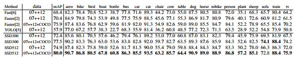
Table 4: PASCAL VOC2012 test detection results. Fast and Faster R-CNN use images with minimum dimension 600, while the image size for YOLO is 448 × 448. data: ”07++12”: union of VOC2007 trainval and test and VOC2012 trainval. ”07++12+COCO”: first train on COCO trainval35k then fine-tune on 07++12.
표 4 : 파스칼 VOC2012 테스트 감지 결과. 신속하고 빠른 R-CNN은 최소 600의 이미지를 사용하고 YOLO의 이미지 크기는 448 × 448입니다. 데이터 : "07 ++ 12": VOC2007 trainval 및 test 및 VOC2012 trainval의 합집합. "07 ++ 12 + COCO": 첫 번째 열차는 COCO trainval 35k에서 07 + 12에서 미세 조정합니다.
3.4 COCO
To further validate the SSD framework, we trained our SSD300 and SSD512 architectures on the COCO dataset. Since objects in COCO tend to be smaller than PASCAL VOC, we use smaller default boxes for all layers. We follow the strategy mentioned in Sec. 2.2, but now our smallest default box has a scale of 0.15 instead of 0.2, and the scale of the default box on conv4 3 is 0.07 (e.g. 21 pixels for a 300 × 300 image)5 .
SSD 프레임 워크를 더욱 검증하기 위해 우리는 COCO 데이터 세트에서 SSD300 및 SSD512 아키텍처를 교육했습니다. COCO의 오브젝트는 PASCAL VOC보다 작기 때문에 모든 레이어에 작은 기본 상자를 사용합니다. 우리는 Sec. 2.2이지만 이제는 가장 작은 기본 상자의 크기가 0.2가 아닌 0.15이고 conv4 3의 기본 상자 크기는 0.07입니다 (예 : 300 × 300 이미지의 경우 21 픽셀).
We use the trainval35k [24] for training. We first train the model with 10−3 learning rate for 160k iterations, and then continue training for 40k iterations with 10−4 and 40k iterations with 10−5 . Table 5 shows the results on test-dev2015. Similar to what we observed on the PASCAL VOC dataset, SSD300 is better than Fast R-CNN in both mAP@0.5 and mAP@[0.5:0.95]. SSD300 has a similar mAP@0.75 as ION [24] and Faster R-CNN [25], but is worse in mAP@0.5. By increasing the image size to 512 × 512, our SSD512 is better than Faster R-CNN [25] in both criteria. Interestingly, we observe that SSD512 is 5.3% better in mAP@0.75, but is only 1.2% better in mAP@0.5. We also observe that it has much better AP (4.8%) and AR (4.6%) for large objects, but has relatively less improvement in AP (1.3%) and AR (2.0%) for small objects. Compared to ION, the improvement in AR for large and small objects is more similar (5.4% vs. 3.9%). We conjecture that Faster R-CNN is more competitive on smaller objects with SSD because it performs two box refinement steps, in both the RPN part and in the Fast R-CNN part. In Fig. 5, we show some detection examples on COCO test-dev with the SSD512 model.
훈련을 위해 trainval35k [24]를 사용합니다. 먼저 160k 반복에 대해 10-3 학습률로 모델을 훈련 한 다음 10-5 및 10-4 및 40k 반복으로 40k 반복 학습을 계속합니다. 표 5는 test-dev2015의 결과를 보여줍니다. PASCAL VOC 데이터 세트에서 관찰 된 것과 유사하게 SSD300은 map@0.5와 mAP @ [0.5 : 0.95]에서 Fast R-CNN보다 우수합니다. SSD300은 ION [24]과 더 빠른 R-CNN [25]과 비슷한 mAP@0.75를 가지고 있지만 mAP@0.5에서는 더 나쁘다. 이미지 크기를 512 × 512로 늘림으로써 SSD512는 두 가지 기준 모두에서 더 빠른 R-CNN [25]보다 낫습니다. 흥미롭게도 우리는 SSD512가 mAP@0.75에서 5.3 % 더 우수하지만 mAP@0.5에서 1.2 % 우수하다는 것을 알 수 있습니다. 또한 대형 물체의 경우 AP (4.8 %)와 AR (4.6 %)가 훨씬 우수하지만 작은 물체의 경우 AP (1.3 %)와 AR (2.0 %)의 개선이 상대적으로 적음을 알 수 있습니다. ION에 비해 크고 작은 물체에 대한 AR의 향상은 더 비슷합니다 (5.4 % 대 3.9 %). RPN 부분과 Fast R-CNN 부분에서 두 개의 상자 세밀화 단계를 수행하기 때문에 더 빠른 R-CNN이 SSD가있는 더 작은 개체에서 더 경쟁력이 있다고 생각합니다. Fig. 5, SSD512 모델의 COCO test-dev에 대한 몇 가지 탐지 예제를 보여줍니다.
3.5 Preliminary ILSVRC results
We applied the same network architecture we used for COCO to the ILSVRC DET dataset [16]. We train a SSD300 model using the ILSVRC2014 DET train and val1 as used in [22]. We first train the model with 10−3 learning rate for 320k iterations, and then continue training for 80k iterations with 10−4 and 40k iterations with 10−5 . We can achieve 43.4 mAP on the val2 set [22]. Again, it validates that SSD is a general framework for high quality real-time detection.
우리는 COCO에서 사용한 것과 동일한 네트워크 아키텍처를 ILSVRC DET 데이터 세트 [16]에 적용했습니다. 우리는 [22]에서 사용 된 ILSVRC2014 DET 트레인과 val1을 사용하여 SSD300 모델을 교육합니다. 먼저 320k 반복에 대해 10-3 학습률로 모델을 훈련시킨 다음 10-5 및 10-4로 40k 반복을 사용하여 80k 반복에 대해 교육을 계속합니다. 우리는 val2 세트에서 43.4 mAP를 달성 할 수 있습니다 [22]. SSD는 고품질의 실시간 탐지를위한 일반적인 프레임 워크임을 다시 한번 입증합니다.
3.6 Data Augmentation for Small Object Accuracy
Without a follow-up feature resampling step as in Faster R-CNN, the classification task for small objects is relatively hard for SSD, as demonstrated in our analysis (see Fig. 4). The data augmentation strategy described in Sec. 2.2 helps to improve the performance dramatically, especially on small datasets such as PASCAL VOC. The random crops generated by the strategy can be thought of as a ”zoom in” operation and can generate many larger training examples. To implement a ”zoom out” operation that creates more small training examples, we first randomly place an image on a canvas of 16× of the original image size filled with mean values before we do any random crop operation. Because we have more training images by introducing this new ”expansion” data augmentation trick, we have to double the training iterations. We have seen a consistent increase of 2%-3% mAP across multiple datasets, as shown in Table 6. In specific, Figure 6 shows that the new augmentation trick significantly improves the performance on small objects. This result underscores the importance of the data augmentation strategy for the final model accuracy.
Faster R-CNN에서와 같이 후속 기능 재 샘플링 단계가 없으면 작은 개체에 대한 분류 작업은 SSD에서 비교적 어렵습니다 (그림 4 참조). Sec.에 기술 된 데이터 증가 전략. 2.2는 특히 PASCAL VOC와 같은 작은 데이터 세트에서 성능을 획기적으로 향상시키는 데 도움이됩니다. 전략에 의해 생성 된 무작위 작물은 "확대 (zoom in)"작업으로 생각할 수 있으며 많은 더 큰 훈련 예제를 생성 할 수 있습니다. 보다 작은 학습 예제를 생성하는 "축소"작업을 구현하기 위해 임의의 자르기 작업을 수행하기 전에 평균 값이 채워진 원본 이미지 크기의 16 배 캔버스에 이미지를 무작위로 배치합니다. 이 새로운 "확장"데이터 증가 트릭을 도입하여 더 많은 교육 이미지를 보유하고 있으므로 교육 반복을 두 배로 늘려야합니다. 표 6에서 볼 수 있듯이 여러 데이터 세트에서 2 % -3 % mAP의 일관된 증가가있었습니다. 특히 그림 6에서는 새로운 증가 트릭이 작은 개체의 성능을 크게 향상시키는 것을 보여줍니다. 이 결과는 최종 모델 정확성을위한 데이터 증가 전략의 중요성을 강조합니다.
An alternative way of improving SSD is to design a better tiling of default boxes so that its position and scale are better aligned with the receptive field of each position on a feature map. We leave this for future work.
SSD를 개선하는 또 다른 방법은 기본 상자의 타일링을보다 잘 설계하여 위치 및 규모가 기능 맵에서 각 위치의 수용 필드와보다 잘 정렬되도록하는 것입니다. 우리는 미래의 작업을 위해 이것을 남겨 둡니다.
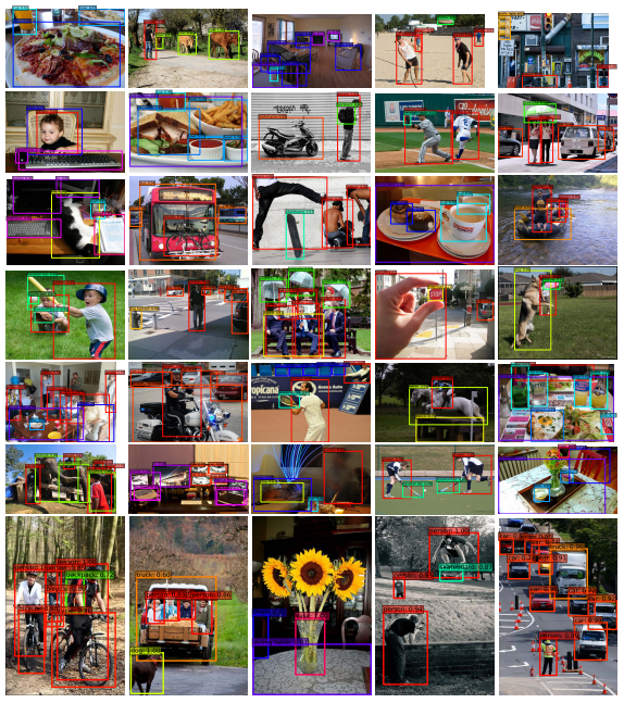
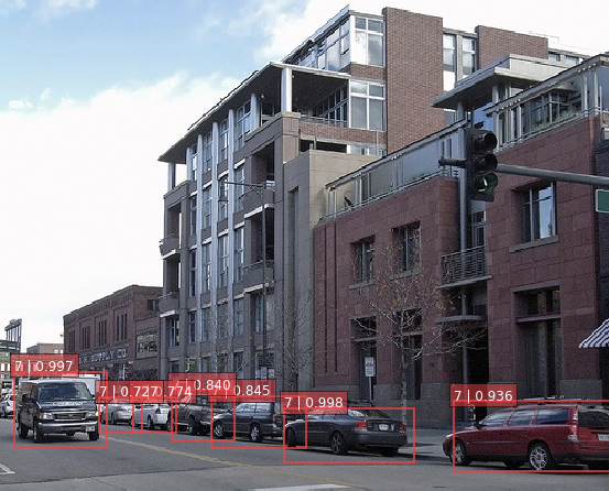
Fig. 5: Detection examples on COCO test-dev with SSD512 model. We show detections with scores higher than 0.6. Each color corresponds to an object category.
그림. 5 : SSD512 모델의 COCO test-dev에 대한 탐지 예제. 우리는 0.6보다 높은 점수로 탐지를 보여줍니다. 각 색상은 객체 카테고리에 해당합니다.

Table 6: Results on multiple datasets when we add the image expansion data augmentation trick. SSD300* and SSD512* are the models that are trained with the new data augmentation.
표 6 : 이미지 확장 데이터 증가 트릭을 추가 할 때 여러 데이터 세트의 결과입니다. SSD300 * 및 SSD512 *는 새로운 데이터 기능을 향상시킨 모델입니다.

Fig. 6: Sensitivity and impact of object size with new data augmentation on VOC2007 test set using [21]. The top row shows the effects of BBox Area per category for the original SSD300 and SSD512 model, and the bottom row corresponds to the SSD300* and SSD512* model trained with the new data augmentation trick. It is obvious that the new data augmentation trick helps detecting small objects significantly.
그림. 6 : [21]을 이용한 VOC2007 테스트 세트의 새로운 데이터 증가와 함께 객체 크기의 민감도와 영향. 맨 위 줄은 원래 SSD300 및 SSD512 모델에 대한 카테고리 당 BBox Area의 효과를 보여 주며 맨 아래 줄은 새로운 데이터 증가 트릭으로 교육 된 SSD300 * 및 SSD512 * 모델에 해당합니다. 새로운 데이터 증가 트릭은 작은 물체를 크게 감지하는 데 도움이됩니다.
3.7 Inference time
Considering the large number of boxes generated from our method, it is essential to perform non-maximum suppression (nms) efficiently during inference. By using a con- fidence threshold of 0.01, we can filter out most boxes. We then apply nms with jaccard overlap of 0.45 per class and keep the top 200 detections per image. This step costs about 1.7 msec per image for SSD300 and 20 VOC classes, which is close to the total time (2.4 msec) spent on all newly added layers. We measure the speed with batch size 8 using Titan X and cuDNN v4 with Intel Xeon E5-2667v3@3.20GHz.
우리의 방법에서 생성 된 많은 수의 상자를 고려할 때, 추론 중에 비 최대 억제 (nms)를 효율적으로 수행하는 것이 필수적이다. 신뢰도 임계 값 0.01을 사용하면 대부분의 상자를 필터링 할 수 있습니다. 우리는 클래스 당 0.45의 jaccard 오버랩을 갖는 nms를 적용하고 이미지 당 최고 200 개의 탐지를 유지합니다. 이 단계는 SSD300 및 20 개의 VOC 클래스에 대해 이미지 당 약 1.7 msec가 소요되며 새로 추가 된 모든 레이어에 소요 된 총 시간 (2.4 msec)에 가깝습니다. Titan X 및 cuDNN v4 (Intel Xeon E5-2667v3@3.20GHz)를 사용하여 배치 크기 8로 속도를 측정합니다.

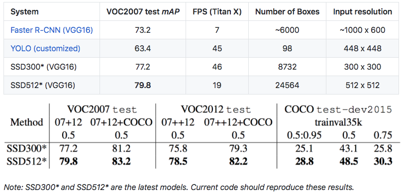
Table 7: Results on Pascal VOC2007 test. SSD300 is the only real-time detection method that can achieve above 70% mAP. By using a larger input image, SSD512 outperforms all methods on accuracy while maintaining a close to real-time speed.
표 7 : 파스칼 VOC2007 테스트 결과 SSD300은 70 % 이상의 mAP를 달성 할 수있는 유일한 실시간 탐지 방법입니다. 더 큰 입력 이미지를 사용함으로써 SSD512는 실시간 속도에 가깝게 유지하면서 정확성에 대한 모든 방법보다 우수한 성능을 보입니다.
Table 7 shows the comparison between SSD, Faster R-CNN[2], and YOLO[5]. Both our SSD300 and SSD512 method outperforms Faster R-CNN in both speed and accuracy. Although Fast YOLO[5] can run at 155 FPS, it has lower accuracy by almost 22% mAP. To the best of our knowledge, SSD300 is the first real-time method to achieve above 70% mAP. Note that about 80% of the forward time is spent on the base network (VGG16 in our case). Therefore, using a faster base network could even further improve the speed, which can possibly make the SSD512 model real-time as well.
표 7은 SSD, 빠른 R-CNN [2], YOLO [5]의 비교를 보여준다. SSD300 및 SSD512 방법 모두 속도와 정확도면에서 빠른 R-CNN보다 우수합니다. Fast Yolo [5]는 155FPS에서 작동 할 수 있지만 거의 22 % mAP만큼 정확도가 떨어집니다. 우리가 아는 한 SSD300은 70 % 이상의 mAP를 달성하는 최초의 실시간 방법입니다. 전달 시간의 약 80 %가 기본 네트워크 (이 경우 VGG16)에 소비된다는 점에 유의하십시오. 따라서 더 빠른 기본 네트워크를 사용하면 속도가 더욱 향상되어 SSD512 모델을 실시간으로 만들 수 있습니다.
4 Related Work
There are two established classes of methods for object detection in images, one based on sliding windows and the other based on region proposal classification. Before the advent of convolutional neural networks, the state of the art for those two approaches – Deformable Part Model (DPM) [26] and Selective Search [1] – had comparable performance. However, after the dramatic improvement brought on by R-CNN [22], which combines selective search region proposals and convolutional network based post-classification, region proposal object detection methods became prevalent.
이미지에서 물체를 탐지하는 방법에는 두 가지 방법이 있습니다. 하나는 슬라이딩 창을 기준으로하고 다른 하나는 지역 제안 분류를 기반으로합니다. 길쌈 신경 네트워크가 출현하기 전에, DPM (Deformable Part Model) [26]과 Selective Search [1]와 같은 두 가지 접근 방식에 대한 기술 수준이 비슷한 성능을 보였습니다. 그러나 선택적인 검색 영역 제안과 컨벌루션 네트워크 기반의 후 분류를 결합한 R-CNN [22]에 의한 극적인 개선 이후에 지역 제안 객체 검출 방법이 널리 보급되었다.
The original R-CNN approach has been improved in a variety of ways. The first set of approaches improve the quality and speed of post-classification, since it requires the classification of thousands of image crops, which is expensive and time-consuming. SPPnet [9] speeds up the original R-CNN approach significantly. It introduces a spatial pyramid pooling layer that is more robust to region size and scale and allows the classification layers to reuse features computed over feature maps generated at several image resolutions. Fast R-CNN [6] extends SPPnet so that it can fine-tune all layers end-toend by minimizing a loss for both confidences and bounding box regression, which was first introduced in MultiBox [7] for learning objectness.
최초의 R-CNN 접근 방식은 다양한 방식으로 향상되었습니다. 첫 번째 접근 방식은 수천 개의 이미지 작물을 분류해야하기 때문에 비용이 많이 소요되고 시간이 오래 걸리기 때문에 분류 작업의 품질과 속도를 향상시킵니다. SPPnet [9]은 원래의 R-CNN 접근법을 상당히 가속화합니다. 영역 크기와 스케일에보다 견고한 공간 피라미드 풀링 레이어를 도입하고 분류 레이어가 여러 이미지 해상도로 생성 된 피쳐 맵을 통해 계산 된 피쳐를 재사용 할 수있게합니다. Fast R-CNN [6]은 SPPnet을 확장하여 객체 박스를 학습하기 위해 MultiBox [7]에서 처음 도입 된 신뢰도 및 경계 상자 회귀에 대한 손실을 최소화하여 모든 계층의 종단점을 미세 조정할 수 있습니다.
The second set of approaches improve the quality of proposal generation using deep neural networks. In the most recent works like MultiBox [7,8], the Selective Search region proposals, which are based on low-level image features, are replaced by proposals generated directly from a separate deep neural network. This further improves the detection accuracy but results in a somewhat complex setup, requiring the training of two neural networks with a dependency between them. Faster R-CNN [2] replaces selective search proposals by ones learned from a region proposal network (RPN), and introduces a method to integrate the RPN with Fast R-CNN by alternating between finetuning shared convolutional layers and prediction layers for these two networks. This way region proposals are used to pool mid-level features and the final classification step is less expensive. Our SSD is very similar to the region proposal network (RPN) in Faster R-CNN in that we also use a fixed set of (default) boxes for prediction, similar to the anchor boxes in the RPN. But instead of using these to pool features and evaluate another classifier, we simultaneously produce a score for each object category in each box. Thus, our approach avoids the complication of merging RPN with Fast R-CNN and is easier to train, faster, and straightforward to integrate in other tasks.
두 번째 접근 방식은 심 신경 네트워크를 사용하여 제안 생성의 품질을 향상시킵니다. MultiBox [7,8]와 같은 가장 최근 연구에서 저급 이미지 특징을 기반으로하는 선택적인 검색 영역 제안은 별도의 심 신경 네트워크에서 직접 생성 된 제안으로 대체되었습니다. 이것은 검출 정확도를 더 향상 시키지만, 다소 복잡한 설정을 초래하며, 두 신경망 사이에 의존성을 갖는 훈련을 필요로한다. 더 빠른 R-CNN [2]은 지역 제안 네트워크 (RPN)에서 배운 것들에 의한 선택적인 검색 제안을 대체하고,이 두 네트워크에 대한 공유 컨벌루션 계층과 예측 계층을 번갈아 가며 RPN을 Fast R-CNN과 통합하는 방법을 소개합니다 . 이 방법으로 지역 제안은 중간 수준 기능을 모으는 데 사용되며 최종 분류 단계는 비교적 저렴합니다. 우리의 SSD는 RPN의 앵커 박스와 유사하게 예측을위한 고정 된 (기본) 박스 세트를 사용한다는 점에서 Faster R-CNN의 RPN (Region Proposal Network)과 매우 유사합니다. 그러나 이러한 기능을 사용하여 기능을 풀고 다른 분류 기준을 평가하는 대신 우리는 동시에 각 상자의 각 객체 범주에 대한 점수를 산출합니다. 따라서 우리의 접근 방식은 Fast R-CNN과 RPN 병합의 복잡성을 피할 수 있으며 훈련하기 쉽고 빠르며 다른 작업에 쉽게 통합 할 수 있습니다.
Another set of methods, which are directly related to our approach, skip the proposal step altogether and predict bounding boxes and confidences for multiple categories directly. OverFeat [4], a deep version of the sliding window method, predicts a bounding box directly from each location of the topmost feature map after knowing the confidences of the underlying object categories. YOLO [5] uses the whole topmost feature map to predict both confidences for multiple categories and bounding boxes (which are shared for these categories). Our SSD method falls in this category because we do not have the proposal step but use the default boxes. However, our approach is more flexible than the existing methods because we can use default boxes of different aspect ratios on each feature location from multiple feature maps at different scales. If we only use one default box per location from the topmost feature map, our SSD would have similar architecture to OverFeat [4]; if we use the whole topmost feature map and add a fully connected layer for predictions instead of our convolutional predictors, and do not explicitly consider multiple aspect ratios, we can approximately reproduce YOLO [5].
우리의 접근 방식과 직접적으로 관련된 또 다른 방법은 제안 단계를 건너 뛰고 여러 범주의 경계 상자와 신뢰도를 직접 예측합니다. 슬라이딩 윈도우 메소드의 심층적 인 버전 인 OverFeat [4]는 기본 객체 카테고리의 신뢰도를 파악한 후 최상위 피쳐 맵의 각 위치에서 직접 경계 상자를 예측합니다. YOLO [5]는 전체 최상위 피쳐 맵을 사용하여 여러 카테고리 및 경계 상자 (이 카테고리에 대해 공유 됨)에 대한 신뢰도를 예측합니다. SSD 방법은 제안 단계가 없기 때문에이 범주에 속하지만 기본 상자를 사용합니다. 그러나 우리의 접근법은 기존의 방법보다 유연합니다. 왜냐하면 다양한 특징 맵에서 각 특징 위치에 다른 비율의 기본 상자를 사용할 수 있기 때문입니다. 최상위 기능 맵에서 위치 당 하나의 기본 상자 만 사용하는 경우 SSD는 OverFeat [4]와 비슷한 아키텍처를가집니다. 우리가 전체 최상위 피쳐 맵을 사용하고 컨볼 루션 예측 자 대신 예측에 대해 완전히 연결된 레이어를 추가하고 여러 종횡비를 명시 적으로 고려하지 않으면 YOLO [5]를 재현 할 수 있습니다.
5 Conclusions
This paper introduces SSD, a fast single-shot object detector for multiple categories. A key feature of our model is the use of multi-scale convolutional bounding box outputs attached to multiple feature maps at the top of the network. This representation allows us to efficiently model the space of possible box shapes. We experimentally validate that given appropriate training strategies, a larger number of carefully chosen default bounding boxes results in improved performance. We build SSD models with at least an order of magnitude more box predictions sampling location, scale, and aspect ratio, than existing methods [5,7]. We demonstrate that given the same VGG-16 base architecture, SSD compares favorably to its state-of-the-art object detector counterparts in terms of both accuracy and speed. Our SSD512 model significantly outperforms the state-of-theart Faster R-CNN [2] in terms of accuracy on PASCAL VOC and COCO, while being 3× faster. Our real time SSD300 model runs at 59 FPS, which is faster than the current real time YOLO [5] alternative, while producing markedly superior detection accuracy.
이 백서에서는 여러 범주에 대한 빠른 단일 샷 객체 감지기 인 SSD를 소개합니다. 우리 모델의 핵심 기능은 네트워크 상단의 여러 기능 맵에 연결된 다중 스케일 컨벌루션 경계 상자 출력을 사용하는 것입니다. 이 표현을 사용하여 가능한 상자 모양의 공간을 효율적으로 모델링 할 수 있습니다. 우리는 적절한 훈련 전략이 주어지면주의 깊게 선택된 기본 경계 상자가 더 많아 질수록 성능이 향상된다는 것을 실험적으로 검증합니다. 우리는 기존 방법 [5,7]보다 위치, 규모 및 종횡비를 샘플링하는 상자 예측보다 더 큰 규모의 SSD 모델을 구축합니다. 우리는 동일한 VGG-16 기본 아키텍처를 제공하므로 SSD는 정확성과 속도 측면에서 최첨단 물체 탐지기와 비교됩니다. 우리의 SSD512 모델은 PASCAL VOC 및 COCO의 정확성 측면에서 최첨단의 Faster R-CNN보다 월등히 뛰어 났지만 3 배 빠릅니다. 우리의 실시간 SSD300 모델은 현존하는 실시간 YOLO [5] 대안보다 더 빠른 59 FPS에서 실행되는 동시에 탁월한 탐지 정확도를 제공합니다.
Apart from its standalone utility, we believe that our monolithic and relatively simple SSD model provides a useful building block for larger systems that employ an object detection component. A promising future direction is to explore its use as part of a system using recurrent neural networks to detect and track objects in video simultaneously.
독립 실행 형 유틸리티와는 별도로 우리는 모 놀리 식의 비교적 간단한 SSD 모델이 객체 감지 구성 요소를 사용하는 대형 시스템에 유용한 빌딩 블록을 제공한다고 믿습니다. 미래의 유망한 방향은 비디오의 객체를 동시에 탐지하고 추적하기 위해 반복적 인 신경망을 사용하는 시스템의 일부로서의 사용을 탐구하는 것입니다.
'MachineLearning' 카테고리의 다른 글
| Bayesian Optimization (2) | 2017.10.31 |
|---|---|
| AUC(Area under an ROC curve)와 ROC (0) | 2017.10.31 |
| YOLO CNN : Real-Time Object Detection (2) | 2017.04.12 |
| SparkNet : Training Deep Networks in Spark (0) | 2017.02.19 |
| Machine Learning with the tools IPython Notebook SFrame (0) | 2017.02.05 |
SSD : Single Shot MultiBox Detector
Reference
Wei Liu1, Dragomir Anguelov2, Dumitru Erhan3, Christian Szegedy3, Scott Reed4, Cheng-Yang Fu1, Alexander C. Berg1
1UNC Chapel Hill 2Zoox Inc. 3Google Inc. 4University of Michigan, Ann-Arbor 1wliu@cs.unc.edu, 2drago@zoox.com, 3{dumitru,szegedy}@google.com, 4reedscot@umich.edu, 1{cyfu,aberg}@cs.unc.edu
https://arxiv.org/abs/1512.02325
ABSTRACT
We present a method for detecting objects in images using a single deep neural network. Our approach, named SSD, discretizes the output space of bounding boxes into a set of default boxes over different aspect ratios and scales per feature map location. At prediction time, the network generates scores for the presence of each object category in each default box and produces adjustments to the box to better match the object shape. Additionally, the network combines predictions from multiple feature maps with different resolutions to naturally handle objects of various sizes. SSD is simple relative to methods that require object proposals because it completely eliminates proposal generation and subsequent pixel or feature resampling stages and encapsulates all computation in a single network. This makes SSD easy to train and straightforward to integrate into systems that require a detection component. Experimental results on the PASCAL VOC, COCO, and ILSVRC datasets confirm that SSD has competitive accuracy to methods that utilize an additional object proposal step and is much faster, while providing a unified framework for both training and inference. For 300 × 300 in- put, SSD achieves 74.3% mAP1 on VOC2007 test at 59 FPS on a Nvidia Titan X and for 512 × 512 input, SSD achieves 76.9% mAP, outperforming a comparable state-of-the-art Faster R-CNN model. Compared to other single stage methods, SSD has much better accuracy even with a smaller input image size. Code is available at: https://github.com/weiliu89/caffe/tree/ssd.
우리는 하나의 심층 신경망 (deep neural network)을 사용하여 이미지의 객체를 검출하는 방법을 제시합니다. SSD라는 이름의 접근 방식은 테두리 상자의 출력 공간을 기능 맵 위치별로 서로 다른 종횡비와 비율로 기본 상자 집합으로 이산합니다. 예측 시간에 네트워크는 각 기본 상자에서 각 개체 범주의 존재에 대한 점수를 생성하고, 개체 모양을 보다 잘 일치시키기 위해 상자를 조정합니다. 또한 네트워크는 다양한 해상도의 여러 기능 맵의 예측을 결합하여 다양한 크기의 개체를 자연스럽게 처리합니다. SSD는 제안서 생성 및 후속 픽셀 또는 기능 재 샘플링 단계를 완전히 제거하고 모든 계산을 단일 네트워크에 캡슐화하기 때문에 객체 제안을 필요로하는 방법에 비해 간단합니다. 이를 통해 SSD는 탐지 구성 요소가 필요한 시스템에 쉽게 통합 할 수 있습니다. PASCAL VOC, COCO 및 ILSVRC 데이터 세트에 대한 실험 결과에 따르면 SSD는 추가 객체 제안 단계를 사용하는 방법과 비교하여 정확성이 뛰어나며 교육(Training)과 추론(Inference) 모두에 통일된 프레임워크를 제공하면서 훨씬 빠릅니다. 300 × 300 입력의 경우 SSD는 Nvidia Titan X에서 59 FPS의 VOC 2007 테스트에서 74.3 % mAP1을 얻었고 512x512 입력의 경우 SSD는 76.9 % mAP를 달성하여 동급 최강의 빠른 R- CNN 모델. 다른 싱글 스테이지 방식에 비해 SSD는 입력 이미지 크기가 작을 때보 다 훨씬 더 정확합니다. 코드는 https://github.com/weiliu89/caffe/tree/ssd에서 사용할 수 있습니다.
Keywords : Real-time Object Detection; Convolutional Neural Network
1 Introduction
Current state-of-the-art object detection systems are variants of the following approach: hypothesize bounding boxes, resample pixels or features for each box, and apply a high- quality classifier. This pipeline has prevailed on detection benchmarks since the Selective Search work [1] through the current leading results on PASCAL VOC, COCO, and ILSVRC detection all based on Faster R-CNN[2] albeit with deeper features such as [3]. While accurate, these approaches have been too computationally intensive for embedded systems and, even with high-end hardware, too slow for real-time applications. Often detection speed for these approaches is measured in seconds per frame (SPF), and even the fastest high-accuracy detector, Faster R-CNN, operates at only 7 frames per second (FPS). There have been many attempts to build faster detectors by attacking each stage of the detection pipeline (see related work in Sec. 4), but so far, significantly increased speed comes only at the cost of significantly decreased detection accuracy.
현재의 최첨단 물체 감지 시스템은 다음과 같은 접근법의 변형입니다 : 경계 상자(bounding boxes)를 가정하고, 각 상자의 픽셀 또는 특징을 재 샘플링하고, 고품질 분류기를 적용합니다. 이 파이프 라인은 PASCAL VOC, COCO 및 ILSVRC 탐지의 최신 결과를 통해 Selective Search 작업 [1] 이후 탐지 벤치 마크에서 우세한 것으로, [3]과 같은 더 깊은 특징이 있음에도 불구하고 빠른 R-CNN을 기반으로합니다 [2]. 이러한 접근 방식은 정확하지만 임베디드 시스템에서는 너무 연산 집약적이었고 고급 하드웨어에서도 실시간 응용 프로그램에는 너무 느립니다. 이러한 접근 방식의 검출 속도는 프레임 당 초 단위 (SPF)로 측정되는 경우가 많으며 가장 빠른 고정밀 검출기 인 Faster R-CNN조차도 초당 7 프레임 (FPS)으로 작동합니다. 탐지 파이프 라인의 각 단계를 공격하여 더 빠른 탐지기를 구축하려는 시도가 많이 있었지만 (4 절의 관련 작업 참조) 지금까지는 감지(detection) 정확도(accuracy)가 현저히 떨어지는 대신 속도가 크게 향상되었습니다.
This paper presents the first deep network based object detector that does not resample pixels or features for bounding box hypotheses and and is as accurate as approaches that do. This results in a significant improvement in speed for high-accuracy detection (59 FPS with mAP 74.3% on VOC2007 test, vs. Faster R-CNN 7 FPS with mAP 73.2% or YOLO 45 FPS with mAP 63.4%). The fundamental improvement in speed comes from eliminating bounding box proposals and the subsequent pixel or feature resampling stage. We are not the first to do this (cf [4,5]), but by adding a series of improvements, we manage to increase the accuracy significantly over previous attempts. Our improvements include using a small convolutional filter to predict object categories and offsets in bounding box locations, using separate predictors (filters) for different aspect ratio detections, and applying these filters to multiple feature maps from the later stages of a network in order to perform detection at multiple scales. With these modifications—especially using multiple layers for prediction at different scales—we can achieve high-accuracy using relatively low resolution input, further increasing detection speed. While these contributions may seem small independently, we note that the resulting system improves accuracy on real-time detection for PASCAL VOC from 63.4% mAP for YOLO to 74.3% mAP for our SSD. This is a larger relative improvement in detection accuracy than that from the recent, very high-profile work on residual networks [3]. Furthermore, significantly improving the speed of high-quality detection can broaden the range of settings where computer vision is useful.
이 논문은 바운딩 박스 가설에 대해 픽셀이나 피쳐를 재 샘플링하지 않는 최초의 딥 네트워크 기반의 객체 검출기를 제시하며, 그러한 접근법만큼 정확합니다. 그 결과 고정밀도 검출 (VOP2007 테스트에서 mAP 74.3 %, mAP 73.2 %를 사용하는 Faster R-CNN 7 FPS 또는 mAP 63.4 %를 사용하는 YOLO 45 FPS)에 비해 속도가 크게 향상되었습니다. 속도의 근본적인 향상은 경계 상자 제안과 후속 픽셀 또는 특징(feature) 리샘플링 단계를 없앰으로써 가능합니다. 우리는 이것을 처음으로하는 것은 아니지만 (cf [4,5]) 일련의 개선 사항을 추가함으로써 이전 시도에 비해 정확성을 크게 높일 수 있습니다. 우리의 개선점으로는 작은 컨볼루션 필터를 사용하여 경계 상자 위치에서 객체 카테고리 및 오프셋을 예측하고, 다른 종횡비 감지에 대해 별도의 예측기(필터)를 사용하고, 네트워크의 후기 단계에서 이러한 필터를 적용하여 수행 할 수 있습니다 여러 척도에서의 탐지. 이러한 수정을 통해 (특히 여러 척도의 예측을 위해 여러 레이어 사용) 상대적으로 낮은 해상도의 입력을 사용하여 고정밀 도로 검색 속도를 높일 수 있습니다. 이러한 기여도는 독립적으로 보일 수 있지만, 결과 시스템은 PASCAL VOC의 실시간 탐지 정확도를 YOLO의 경우 63.4 %에서 SSD의 경우 74.3 %로 향상시킵니다. 이는 잔여 네트워크에 대한 최근의 매우 중요한 작업에서보다 탐지 정확도에서 더 큰 상대적인 향상이다 [3]. 또한 고품질 감지 속도를 크게 향상 시키면 컴퓨터 비전이 유용한 설정 범위를 넓힐 수 있습니다.
We summarize our contributions as follows:
We introduce SSD, a single-shot detector for multiple categories that is faster than the previous state-of-the-art for single shot detectors (YOLO), and significantly more accurate, in fact as accurate as slower techniques that perform explicit region proposals and pooling (including Faster R-CNN).
The core of SSD is predicting category scores and box offsets for a fixed set of default bounding boxes using small convolutional filters applied to feature maps. To achieve high detection accuracy we produce predictions of different scales from feature maps of different scales, and explicitly separate predictions by aspect ratio. These design features lead to simple end-to-end training and high accuracy, even on low resolution input images, further improving the speed vs accuracy trade-off. Experiments include timing and accuracy analysis on models with varying input size evaluated on PASCAL VOC, COCO, and ILSVRC and are compared to a range of recent state-of-the-art approaches.
우리는 우리의 공헌을 다음과 같이 요약합니다 :
우리는 싱글 샷 검출기(YOLO)에 대한 이전의 최첨단 기술보다 더 빠른 여러 범주의 단일 샷 검출기 인 SSD를 소개하고 명시 적 영역 제안을 수행하는 더 느린 기술만큼 정확하고 훨씬 정확합니다 및 풀링 (빠른 R-CNN 포함).
SSD의 핵심은 기능 맵에 적용된 작은 컨볼 루션 필터를 사용하여 고정 된 기본 경계 상자 집합에 대한 범주 점수 및 상자 오프셋을 예측하는 것입니다. 높은 탐지 정확도를 달성하기 위해 서로 다른 스케일의 기능 맵과 다른 스케일의 예측을 생성하고 명시 적으로 종횡비별로 예측을 분리합니다. 이러한 디자인 기능은 저해상도 입력 이미지 에서조차 간단한 엔드 투 엔드 (end-to-end) 교육과 높은 정확도를 제공하여 속도와 정확도의 균형을 더욱 향상시킵니다. 실험에는 PASCAL VOC, COCO 및 ILSVRC에서 평가되는 다양한 입력 크기를 가진 모델에 대한 타이밍 및 정확도 분석이 포함되며 최근의 최첨단 접근 방식과 비교됩니다.
2 The Single Shot Detector (SSD)
This section describes our proposed SSD framework for detection (Sec. 2.1) and the associated training methodology (Sec. 2.2). Afterwards, Sec. 3 presents dataset-specific model details and experimental results.
이 절에서는 제안 된 SSD 탐지 프레임 워크 (2.1 절)와 관련 교육 방법론 (2.2 절)에 대해 설명합니다. 그 후에, Sec. 3은 데이터 집합 별 모델 세부 정보 및 실험 결과를 나타냅니다.
Fig. 1: SSD framework. (a) SSD only needs an input image and ground truth boxes for each object during training. In a convolutional fashion, we evaluate a small set (e.g. 4) of default boxes of different aspect ratios at each location in several feature maps with different scales (e.g. 8 × 8 and 4 × 4 in (b) and (c)). For each default box, we predict both the shape offsets and the confidences for all object categories ((c1 , c2 , · · · , cp )). At training time, we first match these default boxes to the ground truth boxes. For example, we have matched two default boxes with the cat and one with the dog, which are treated as positives and the rest as negatives. The model loss is a weighted sum between localization loss (e.g. Smooth L1 [6]) and confidence loss (e.g. Softmax).
그림. 1 : SSD 프레임 워크. (a) SSD는 훈련 중 각 물체에 대한 입력 이미지 및 접지 진실 상자 만 필요합니다. 컨벌루션 방식으로, 우리는 다른 측면 여러 특징 맵의 각 위치에서 다른 화면 비율의 기본 상자의 작은 세트를 (예를 들어, 4) 평가 (예를 들어, 8 × 8, 4 × 4 (b)와 (c)). 각 기본 상자, 우리는 모양 오프셋 및 모든 개체 종류에 대한 비밀도 ((C1, C2, · · ·, CP))를 모두 예측하고있다. 교육 시간에, 우리는 먼저이 기본 상자를 지상 진실 상자와 일치시킵니다. 예를 들어, 우리는 긍정과 부정과 나머지로 취급되는 두 개의 기본 고양이와 상자와 개를, 일치했다. 모델 손실 파악 손실 (예를 들어 부드러운 L1 [6])와 지수 손실 (예를 들어, 소프트 맥스) 사이의 가중된 합이다.
2.1 Model
The SSD approach is based on a feed-forward convolutional network that produces a fixed-size collection of bounding boxes and scores for the presence of object class instances in those boxes, followed by a non-maximum suppression step to produce the final detections. The early network layers are based on a standard architecture used for high quality image classification (truncated before any classification layers), which we will call the base network2. We then add auxiliary structure to the network to produce detections with the following key features:
SSD 접근 방식은 고정 박스 크기의 경계 상자 모음과 해당 상자에있는 개체 클래스 인스턴스의 존재 여부에 대한 점수를 생성하는 피드 포워드 컨볼 루션 네트워크를 기반으로하며 최종 탐지를 생성하는 비 최대 억제 단계가 뒤 따른다. 초기 네트워크 계층은 고품질 이미지 분류 (모든 분류 계층 전에 절단 됨)에 사용되는 표준 아키텍처를 기반으로하며이를 기본 네트워크 2라고합니다. 그런 다음 네트워크에 보조 구조를 추가하여 다음과 같은 주요 기능을 갖춘 탐지를 생성합니다.
Multi-scale feature maps for detection We add convolutional feature layers to the end of the truncated base network. These layers decrease in size progressively and allow predictions of detections at multiple scales. The convolutional model for predicting detections is different for each feature layer (cf Overfeat[4] and YOLO[5] that operate on a single scale feature map).
탐지를 위한 다중 스케일 피쳐 맵 절단 된 기본 네트워크의 끝에 컨볼 루션 피쳐 레이어를 추가합니다. 이러한 레이어는 점진적으로 크기가 감소하고 여러 배율에서 감지를 예측할 수 있습니다. 탐지를 예측하기위한 컨볼 루션 모델은 각 기능 레이어마다 다릅니다 (단일 배율 피쳐 맵에서 작동하는 Overfeat [4] 및 YOLO [5] 참조).
Convolutional predictors for detection Each added feature layer (or optionally an existing feature layer from the base network) can produce a fixed set of detection predictions using a set of convolutional filters. These are indicated on top of the SSD network architecture in Fig. 2. For a feature layer of size m × n with p channels, the basic element for predicting parameters of a potential detection is a 3 × 3 × p small kernel that produces either a score for a category, or a shape offset relative to the default box coordinates. At each of the m × n locations where the kernel is applied, it produces an output value. The bounding box offset output values are measured relative to a default box position relative to each feature map location (cf the architecture of YOLO[5] that uses an intermediate fully connected layer instead of a convolutional filter for this step).
탐지를위한 컨벌루션 예측자 추가된 각 피쳐 레이어 (또는 선택적으로 기본 네트워크의 기존 피쳐 레이어)는 컨벌루션 필터 세트를 사용하여 고정 된 탐지 예측 세트를 생성 할 수 있습니다. 이는 그림 1의 SSD 네트워크 아키텍처의 상단에 표시됩니다. 2. p 채널을 갖는 크기 m × n의 Feature 레이어의 경우, 잠재적 인 검출의 매개 변수를 예측하기위한 기본 요소는 범주에 대한 점수를 산출하는 3x3xp의 작은 커널 또는 기본 상자 좌표. 커널이 적용되는 mxn 위치 각각에서 출력 값을 생성합니다. 바운딩 박스 오프셋 출력 값은 각 Feature 맵 위치와 관련된 기본 상자 위치에 상대적으로 측정됩니다 (이 단계에서 컨벌루션 필터 대신 중간 완전 연결 레이어를 사용하는 YOLO [5] 아키텍처 참조).
Fig. 2: A comparison between two single shot detection models: SSD and YOLO [5]. Our SSD model adds several feature layers to the end of a base network, which predict the offsets to default boxes of different scales and aspect ratios and their associated confidences. SSD with a 300 × 300 input size significantly outperforms its 448 × 448 YOLO counterpart in accuracy on VOC2007 test while also improving the speed.
그림. 2 : 두 개의 단일 샷 검출 모델 인 SSD와 YOLO [5]의 비교. 우리의 SSD 모델은 기본 네트워크의 끝 부분에 몇 가지 기능 레이어를 추가합니다.이 기능 레이어는 서로 다른 크기와 종횡비 및 관련 신뢰도의 기본 상자에 대한 오프셋을 예측합니다. 300 × 300 입력 크기의 SSD는 VOC2007 테스트의 정확도에서 448 × 448 YOLO 성능보다 월등히 뛰어남과 동시에 속도가 향상되었습니다.
Default boxes and aspect ratios We associate a set of default bounding boxes with each feature map cell, for multiple feature maps at the top of the network. The default boxes tile the feature map in a convolutional manner, so that the position of each box relative to its corresponding cell is fixed. At each feature map cell, we predict the offsets relative to the default box shapes in the cell, as well as the per-class scores that indicate the presence of a class instance in each of those boxes. Specifically, for each box out of k at a given location, we compute c class scores and the 4 offsets relative to the original default box shape. This results in a total of (c + 4)k filters that are applied around each location in the feature map, yielding (c + 4)kmn outputs for a m × n feature map. For an illustration of default boxes, please refer to Fig. 1. Our default boxes are similar to the anchor boxes used in Faster R-CNN [2], however we apply them to several feature maps of different resolutions. Allowing different default box shapes in several feature maps let us efficiently discretize the space of possible output box shapes.
기본 상자 및 가로 세로 비율 기본 테두리 상자 세트를 각 기능 맵 셀과 연결하여 네트워크 맨 위에있는 여러 기능 맵을 찾습니다. 기본 상자는 기능 맵을 컨볼 루션 방식으로 배열하여 각 상자의 해당 셀에 대한 위치가 고정되도록합니다. 각 피쳐 지도 셀에서 셀의 기본 상자 모양과 관련된 오프셋과 각 상자에 클래스 인스턴스가 있음을 나타내는 클래스 별 점수를 예측합니다. 특히 주어진 위치에서 k의 각 상자에 대해 원래의 기본 상자 모양과 관련하여 c 클래스 점수와 4 개의 오프셋을 계산합니다. 그 결과, (c + 4) k 개의 필터가 기능 맵의 각 위치 주변에 적용되어 m × n 피쳐 맵에 대해 (c + 4) kmn 출력을 산출합니다. 기본 상자에 대한 설명은 그림 2를 참조하십시오. 1. 우리의 기본 박스는 Faster R-CNN [2]에서 사용 된 앵커 박스와 비슷하지만 해상도가 다른 여러 개의 기능 맵에 적용합니다. 여러 가지 기능 맵에서 다른 기본 상자 모양을 허용하면 가능한 출력 상자 모양의 공간을 효율적으로 분리 할 수 있습니다.
2.2 Training
The key difference between training SSD and training a typical detector that uses region proposals, is that ground truth information needs to be assigned to specific outputs in the fixed set of detector outputs. Some version of this is also required for training in YOLO[5] and for the region proposal stage of Faster R-CNN[2] and MultiBox[7]. Once this assignment is determined, the loss function and backpropagation are applied end- to-end. Training also involves choosing the set of default boxes and scales for detection as well as the hard negative mining and data augmentation strategies.
SSD 교육과 지역 제안서를 사용하는 일반적인 탐지기 교육의 주요 차이점은 지상 진실 정보를 고정 된 감지기 출력 세트의 특정 출력에 할당해야한다는 것입니다. 이 중 일부 버전은 YOLO [5]의 교육 및 Faster R-CNN [2] 및 MultiBox [7]의 지역 제안 단계에도 필요합니다. 일단이 할당이 결정되면, 손실 함수 및 역 전파가 종단 간 적용됩니다. 또한 교육에는 하드 네거티브 마이닝 및 데이터 확대 전략뿐 아니라 탐지 용 기본 상자 및 눈금 세트 선택이 포함됩니다.
Matching strategy During training we need to determine which default boxes correspond to a ground truth detection and train the network accordingly. For each ground truth box we are selecting from default boxes that vary over location, aspect ratio, and scale. We begin by matching each ground truth box to the default box with the best jaccard overlap (as in MultiBox [7]). Unlike MultiBox, we then match default boxes to any ground truth with jaccard overlap higher than a threshold (0.5). This simplifies the learning problem, allowing the network to predict high scores for multiple overlapping default boxes rather than requiring it to pick only the one with maximum overlap.
일치하는 전략 훈련 중 우리는 지상실 진위 감지에 해당하는 기본 상자를 판별하고 이에 따라 네트워크를 훈련해야합니다. 각 지상 진실 상자에 대해 우리는 위치, 종횡비 및 규모에 따라 다른 기본 상자에서 선택합니다. 우선 각 진실 상자를 가장 좋은 jaccard가 겹치는 기본 상자에 일치 시켜서 시작합니다 (MultiBox [7] 에서처럼). MultiBox와는 달리 임계 값 (0.5)보다 높은 jaccard 겹침을 사용하여 기본 상자를 접지 진리와 일치시킵니다. 이것은 학습 문제를 단순화하여, 네트워크가 최대 겹침이있는 것을 선택하도록 요구하지 않고, 다수의 겹쳐진 디폴트 박스에 대한 높은 점수를 예측할 수있게한다.
Training objective The SSD training objective is derived from the MultiBox objective[7,8]but is extended to handle multiple object categories. Let xpij ={1,0} be an indicator for matching the i-th default box to the j-th ground truth box of category p. In the matching strategy above, we can have i xpij ≥ 1. The overall objective loss function is a weighted sum of the localization loss (loc) and the confidence loss (conf):
교육 목표 SSD 교육 목표는 MultiBox 목표 [7,8]에서 파생되었지만 여러 객체 카테고리를 처리하도록 확장되었습니다. xpij = {1,0}을 i 번째 기본 상자를 범주 p의 j 번째 접지 상자에 일치시키는 지표로 둡니다. 위의 매칭 전략에서, 우리는 i xpij ≥ 1을 가질 수있다. 전반적인 목표 손실 함수는 위치 파악 손실 (loc)과 신뢰 손실 (conf)의 가중치 합이다.
where N is the number of matched default boxes. If N = 0, wet set the loss to 0. The localization loss is a Smooth L1 loss [6] between the predicted box (l) and the ground truth box (g) parameters. Similar to Faster R-CNN [2], we regress to offsets for the center (cx, cy) of the default bounding box (d) and for its width (w) and height (h).
여기서 N은 일치하는 기본 상자의 수입니다. N = 0이면 손실을 0으로 설정합니다. 위치 파악 손실은 예측 상자 (l)와 접지 실 상자 (g) 매개 변수 사이의 부드러운 L1 손실입니다 [6]. Faster R-CNN [2]과 마찬가지로 기본 경계 상자 (d)의 중심 (cx, cy)과 폭 (w) 및 높이 (h)에 대한 오프셋으로 회귀합니다.
The confidence loss is the softmax loss over multiple classes confidences (c).
신뢰 손실은 여러 클래스 신뢰도 (c)에 대한 softmax 손실입니다.
and the weight term α is set to 1 by cross validation.
교차 검증에 의해 가중 항 α가 1로 설정된다.
Choosing scales and aspect ratios for default boxes To handle different object scales, some methods [4,9] suggest processing the image at different sizes and combining the results afterwards. However, by utilizing feature maps from several different layers in a single network for prediction we can mimic the same effect, while also sharing parameters across all object scales. Previous works [10,11] have shown that using feature maps from the lower layers can improve semantic segmentation quality because the lower layers capture more fine details of the input objects. Similarly, [12] showed that adding global context pooled from a feature map can help smooth the segmentation results. Motivated by these methods, we use both the lower and upper feature maps for detection. Figure 1 shows two exemplar feature maps (8 × 8 and 4 × 4) which are used in the framework. In practice, we can use many more with small computational overhead.
기본 상자의 비율 및 종횡비 선택 서로 다른 객체 크기를 처리하기 위해 일부 방법 [4,9]에서는 이미지를 다른 크기로 처리하고 나중에 결과를 결합하는 것이 좋습니다. 그러나 예측을 위해 단일 네트워크에서 여러 레이어의 기능 맵을 활용함으로써 동일한 효과를 모방하고 모든 객체 척도에서 매개 변수를 공유 할 수 있습니다. 이전 연구 [10,11]에서는 하위 계층이 입력 객체의 세부 묘사를 더 잘 포착하기 때문에 하위 계층의 특성 맵을 사용하면 의미론적 세분화 품질을 향상시킬 수 있다는 것을 보여주었습니다. 유사하게, [12]는 feature map으로부터 풀링 된 global context를 추가하는 것이 segmentation 결과를 부드럽게하는데 도움을 줄 수 있음을 보였다. 이 방법들에 의해 동기 부여를 위해 우리는 탐지를 위해 하부 및 상부 특징 맵 모두를 사용한다. 그림 1은 프레임 워크에서 사용되는 두 개의 표본 피쳐 맵 (8 × 8 및 4 × 4)을 보여줍니다. 실제로는 적은 계산 오버 헤드로 더 많은 것을 사용할 수 있습니다.
Feature maps from different levels within a network are known to have different (empirical) receptive field sizes [13]. Fortunately, within the SSD framework, the de- fault boxes do not necessary need to correspond to the actual receptive fields of each layer. We design the tiling of default boxes so that specific feature maps learn to be responsive to particular scales of the objects. Suppose we want to use m feature maps for prediction. The scale of the default boxes for each feature map is computed as:
네트워크 내의 서로 다른 레벨의 특성 맵은 서로 다른 (경험적) 수용 필드 크기를 갖는 것으로 알려져있다 [13]. 다행스럽게도 SSD 프레임 워크 내에서 기본 상자는 각 계층의 실제 수용 필드와 일치 할 필요는 없습니다. 특정 기능 맵이 객체의 특정 축척에 반응하는 것을 배우도록 기본 상자의 기와(tiling)를 디자인합니다. 예측을 위해 m 개의 피처 맵을 사용한다고 가정합니다. 각 기능 맵의 기본 상자 크기는 다음과 같이 계산됩니다.
where smin is 0.2 and smax is 0.9, meaning the lowest layer has a scale of 0.2 and the highest layer has a scale of 0.9, and all layers in between are regularly spaced. We impose different aspect ratios for the default boxes, and denote them as ar ∈ {1, 2, 3, 1 2 , 1 3 }. We can compute the width (w a k = sk √ ar) and height (h a k = sk/ √ ar) for each default box. For the aspect ratio of 1, we also add a default box whose scale is s 0 k = √sksk+1, resulting in 6 default boxes per feature map location. We set the center of each default box to ( i+0.5 |fk| , j+0.5 |fk| ), where |fk| is the size of the k-th square feature map, i, j ∈ [0, |fk|). In practice, one can also design a distribution of default boxes to best fit a specific dataset. How to design the optimal tiling is an open question as well.
smin이 0.2이고 smax가 0.9 인 경우 가장 낮은 레이어는 0.2의 눈금을 가지며 가장 높은 레이어는 0.9의 눈금을 가지며 그 사이의 모든 레이어는 규칙적으로 간격을두고 있습니다. 우리는 디폴트 박스들에 대해 다른 종횡비를 부과하고 그것들을 ar ∈ {1, 2, 3, 1 2, 1 3}로 표시한다. 각 기본 상자의 너비 (w a k = sk √ ar)와 높이 (h a k = sk / √ ar)를 계산할 수 있습니다. 종횡비가 1 인 경우 축척이 s 0 k = √ sksk + 1 인 기본 상자를 추가하여 피쳐지도 위치 당 6 개의 기본 상자가 생성됩니다. 각 기본 상자의 중심을 (i + 0.5 | fk |, j + 0.5 | fk |)로 설정합니다. 여기서 | fk | 는 k 번째 사각형 특징 맵의 크기, i, j ∈ [0, | fk |)이다. 실제로는 특정 데이터 세트에 가장 잘 맞는 기본 상자를 디자인 할 수도 있습니다. 최적의 타일링을 설계하는 방법도 공개적인 질문입니다.
By combining predictions for all default boxes with different scales and aspect ratios from all locations of many feature maps, we have a diverse set of predictions, covering various input object sizes and shapes. For example, in Fig. 1, the dog is matched to a default box in the 4 × 4 feature map, but not to any default boxes in the 8 × 8 feature map. This is because those boxes have different scales and do not match the dog box, and therefore are considered as negatives during training.
모든 기본 기능 상자에 대한 예측을 여러 기능 맵의 모든 위치에서 다른 비율 및 종횡비로 결합하여 다양한 입력 개체 크기 및 모양을 포괄하는 다양한 예측을 제공합니다. 예를 들어, Fig. 1이면 개가 4x4 기능 맵에서 기본 상자와 일치하지만 8x8 기능 맵에서는 기본 상자와 일치하지 않습니다. 이러한 상자는 다른 크기와 도그 박스와 일치하지 않기 때문에 훈련 중에 네거티브로 간주되기 때문입니다.
Hard negative mining After the matching step, most of the default boxes are negatives, especially when the number of possible default boxes is large. This introduces a significant imbalance between the positive and negative training examples. Instead of using all the negative examples, we sort them using the highest confidence loss for each default box and pick the top ones so that the ratio between the negatives and positives is at most 3:1. We found that this leads to faster optimization and a more stable training.
단점 마이닝 (Hard Negative mining) 매칭 단계가 끝나면 기본 상자의 대부분이 네거티브이며, 특히 가능한 기본 상자 수가 많으면 특히 그렇습니다. 이것은 긍정적 인 것과 부정적인 훈련의 예들 사이에 상당한 불균형을 가져온다. 모든 음화 예제를 사용하는 대신, 각 기본 상자에 대해 가장 높은 신뢰도 손실을 사용하여 정렬하고 음수와 양수 비율이 3 : 1 이하가되도록 상위 상자를 선택합니다. 우리는 이것이보다 빠른 최적화와보다 안정적인 교육을 유도한다는 것을 발견했습니다.
Data augmentation To make the model more robust to various input object sizes and shapes, each training image is randomly sampled by one of the following options:
데이터 증가 다양한 입력 개체 크기 및 모양에 대한 모델을보다 강력하게 만들기 위해 각 교육 이미지는 다음 옵션 중 하나에 의해 무작위로 샘플링됩니다.
– Use the entire original input image.
– Sample a patch so that the minimum jaccard overlap with the objects is 0.1, 0.3, 0.5, 0.7, or 0.9.
- Randomly sample a patch.
- 원본 입력 이미지 전체를 사용하십시오.
- 최소 jaccard가 오브젝트와 겹치도록 패치를 샘플링하여 0.1, 0.3, 0.5, 0.7 또는 0.9가되도록하십시오.
- 무작위로 패치를 샘플링하십시오.
The size of each sampled patch is [0.1, 1] of the original image size, and the aspect ratio is between 1 2 and 2. We keep the overlapped part of the ground truth box if the center of it is in the sampled patch. After the aforementioned sampling step, each sampled patch is resized to fixed size and is horizontally flipped with probability of 0.5, in addition to applying some photo-metric distortions similar to those described in [14].
샘플링 된 각 패치의 크기는 원본 이미지 크기의 [0.1, 1]이고 종횡비는 1 2 2입니다. 중심이 샘플링 된 패치에있는 경우 지상 진실 상자의 중첩 된 부분을 유지합니다. 앞서 언급 한 샘플링 단계 후에 샘플링 된 각 패치는 고정 크기로 크기가 조정되고 [14]에서 설명한 것과 유사한 몇 가지 사진 메트릭 왜곡을 적용 할뿐만 아니라 0.5의 확률로 수평으로 대칭 이동됩니다.
3 Experimental Results
Base network Our experiments are all based on VGG16 [15], which is pre-trained on the ILSVRC CLS-LOC dataset [16]. Similar to DeepLab-LargeFOV [17], we convert fc6 and fc7 to convolutional layers, subsample parameters from fc6 and fc7, change pool5 from 2 × 2 − s2 to 3 × 3 − s1, and use the a trous ` algorithm [18] to fill the ”holes”. We remove all the dropout layers and the fc8 layer. We fine-tune the resulting model using SGD with initial learning rate 10−3 , 0.9 momentum, 0.0005 weight decay, and batch size 32. The learning rate decay policy is slightly different for each dataset, and we will describe details later. The full training and testing code is built on Caffe [19] and is open source at: https://github.com/weiliu89/caffe/tree/ssd.
기본 네트워크 우리의 실험은 모두 ILSVRC CLS-LOC 데이터 세트 [16]에 사전 교육 된 VGG16 [15]을 기반으로합니다. DeepLab-LargeFOV [17]와 마찬가지로, fc6와 fc7을 convolutional layer로 변환하고, fc6와 fc7의 서브 샘플 파라미터를 2x2 - s2에서 3x3 - s1로 변경하고, trous 알고리즘 [18] "구멍"을 채우기 위해. 우리는 모든 드롭 아웃 레이어와 fc8 레이어를 제거합니다. SGD를 사용하여 결과 모델을 초기 학습 속도 10-3, 0.9 운동량, 0.0005 무게 감소 및 배치 크기 32로 미세 조정합니다. 학습 속도 감소 정책은 각 데이터 세트마다 약간 씩 다르며 나중에 자세히 설명 할 것입니다. 전체 교육 및 테스트 코드는 Caffe [19]를 기반으로하며 https://github.com/weiliu89/caffe/tree/ssd에서 공개 소스입니다.
3.1 PASCAL VOC2007
On this dataset, we compare against Fast R-CNN [6] and Faster R-CNN [2] on VOC2007 test (4952 images). All methods fine-tune on the same pre-trained VGG16 network.
이 데이터 세트에서 VOC2007 테스트 (4952 개 이미지)에서 Fast R-CNN [6]과 Faster R-CNN [2]을 비교합니다. 모든 방법은 동일한 사전 훈련 된 VGG16 네트워크를 미세 조정합니다.
Figure 2 shows the architecture details of the SSD300 model. We use conv4 3, conv7 (fc7), conv8 2, conv9 2, conv10 2, and conv11 2 to predict both location and confidences. We set default box with scale 0.1 on conv4 3 3 . We initialize the parameters for all the newly added convolutional layers with the ”xavier” method [20]. For conv4 3, conv10 2 and conv11 2, we only associate 4 default boxes at each feature map location – omitting aspect ratios of 1 3 and 3. For all other layers, we put 6 default boxes as described in Sec. 2.2. Since, as pointed out in [12], conv4 3 has a different feature scale compared to the other layers, we use the L2 normalization technique introduced in [12] to scale the feature norm at each location in the feature map to 20 and learn the scale during back propagation. We use the 10−3 learning rate for 40k iterations, then continue training for 10k iterations with 10−4 and 10−5 . When training on VOC2007 trainval, Table 1 shows that our low resolution SSD300 model is already more accurate than Fast R-CNN. When we train SSD on a larger 512 × 512 input image, it is even more accurate, surpassing Faster R-CNN by 1.7% mAP. If we train SSD with more (i.e. 07+12) data, we see that SSD300 is already better than Faster R-CNN by 1.1% and that SSD512 is 3.6% better. If we take models trained on COCO trainval35k as described in Sec. 3.4 and fine-tuning them on the 07+12 dataset with SSD512, we achieve the best results: 81.6% mAP
그림 2는 SSD300 모델의 아키텍처 세부 정보를 보여줍니다. conv4 3, conv7 (fc7), conv8 2, conv9 2, conv10 2 및 conv11 2를 사용하여 위치와 신뢰도를 모두 예측합니다. conv4 3의 scale 0.1로 default box를 설정합니다. 3 3. "xavier"방법 [20]을 사용하여 새로 추가 된 모든 컨볼 루션 계층에 대한 매개 변수를 초기화합니다. conv4 3, conv10 2 및 conv11 2의 경우, 각 기능 맵 위치에 4 개의 기본 상자 만 연결합니다. 1-3 및 3의 종횡비는 생략합니다. 다른 모든 레이어의 경우 6 단계에서 설명한대로 6 개의 기본 상자를 넣습니다. 2.2. [12]에서 지적했듯이, conv4 3은 다른 계층에 비해 다른 특징 규모를 가지고 있기 때문에, [12]에서 소개 된 L2 정규화 기법을 사용하여 feature map의 각 위치에서의 feature norm을 20으로 스케일링하고 역 전파 중에 규모. 우리는 40-3 번의 반복에 대해 10-3 학습률을 사용하고 10-4 및 10-5로 10k 반복에 대한 학습을 계속합니다. VOC2007 trainval을 교육 할 때, 표 1은 우리의 저해상도 SSD300 모델이 이미 Fast R-CNN보다 더 정확하다는 것을 보여줍니다. 더 큰 512 × 512 입력 이미지에서 SSD를 학습 할 때, 훨씬 더 정확하여 빠른 R-CNN을 1.7 % mAP 능가합니다. 더 많은 (즉, 07 + 12) 데이터로 SSD를 교육하면 SSD300이 이미 Faster R-CNN보다 1.1 % 더 좋고 SSD512가 3.6 % 더 우수하다는 것을 알 수 있습니다. 우리가 COCO trainval 35k에서 훈련 된 모델을 Sec. 3.4와 SSD512로 07 + 12 데이터 세트에서 미세 조정하면 최상의 결과를 얻을 수 있습니다 : 81.6 % mAP.
To understand the performance of our two SSD models in more details, we used the detection analysis tool from [21]. Figure 3 shows that SSD can detect various object categories with high quality (large white area). The majority of its confident detections are correct. The recall is around 85-90%, and is much higher with “weak” (0.1 jaccard overlap) criteria. Compared to R-CNN [22], SSD has less localization error, indicating that SSD can localize objects better because it directly learns to regress the object shape and classify object categories instead of using two decoupled steps. However, SSD has more confusions with similar object categories (especially for animals), partly because we share locations for multiple categories. Figure 4 shows that SSD is very sensitive to the bounding box size. In other words, it has much worse performance on smaller objects than bigger objects. This is not surprising because those small objects may not even have any information at the very top layers. Increasing the input size (e.g. from 300×300 to 512×512) can help improve detecting small objects, but there is still a lot of room to improve. On the positive side, we can clearly see that SSD performs really well on large objects. And it is very robust to different object aspect ratios because we use default boxes of various aspect ratios per feature map location.
두 개의 SSD 모델의 성능을보다 자세히 이해하기 위해 [21]의 탐지 분석 도구를 사용했습니다. 그림 3은 SSD가 고품질 (큰 흰색 영역)의 다양한 객체 카테고리를 탐지 할 수 있음을 보여줍니다. 자체 탐지의 대부분은 정확합니다. 리콜은 약 85-90 %이며 "약한"(0.1 jaccard overlap) 기준으로 훨씬 높습니다. R-CNN [22]과 비교할 때 SSD는 지역화 오류가 적기 때문에 SSD는 두 개의 분리 된 단계를 사용하는 대신 객체 모양을 회귀하고 객체 범주를 직접 배울 수 있기 때문에 객체를 더 잘 지역화 할 수 있습니다. 그러나 SSD는 유사한 객체 카테고리 (특히 동물)와 더 많은 혼란을 빚고 있습니다. 부분적으로는 여러 카테고리에 대한 위치를 공유하기 때문입니다. 그림 4는 SSD가 테두리 상자 크기에 매우 민감하다는 것을 보여줍니다. 즉, 더 작은 물체는 큰 물체보다 훨씬 더 나쁜 성능을 보입니다. 이러한 작은 오브젝트는 맨 위의 레이어에 정보가 없기 때문에 놀라운 것은 아닙니다. 입력 크기를 늘리면 (예 : 300 × 300에서 512 × 512로) 작은 물체를 감지하는 데 도움이 될 수 있지만 개선해야 할 부분이 많이 남아 있습니다. 긍정적 인 측면에서 볼 때 SSD가 큰 개체에서 실제로 잘 수행되는지 확인할 수 있습니다. 또한 기능 맵 위치마다 다양한 종횡비의 기본 상자를 사용하기 때문에 다양한 오브젝트 종횡비에 매우 강력합니다.
Table 1: PASCAL VOC2007 test detection results. Both Fast and Faster R-CNN use input images whose minimum dimension is 600. The two SSD models have exactly the same settings except that they have different input sizes (300×300 vs. 512×512). It is obvious that larger input size leads to better results, and more data always helps. Data: ”07”: VOC2007 trainval, ”07+12”: union of VOC2007 and VOC2012 trainval. ”07+12+COCO”: first train on COCO trainval35k then fine-tune on 07+12.
표 1 : PASCAL VOC2007 테스트 감지 결과. 빠른 속도와 빠른 R-CNN은 최소 치수가 600 인 입력 이미지를 사용합니다. 두 SSD 모델은 입력 크기가 서로 다른 것을 제외하고는 정확히 동일한 설정을 사용합니다 (300 × 300 대 512 × 512). 입력 크기가 커지면 결과가 더 좋아지고 데이터가 많을수록 항상 도움이됩니다. 데이터 : "07": VOC2007 trainval, "07 + 12": VOC2007 및 VOC2012 trainval의 조합. "07 + 12 + COCO": 첫 번째 열차는 COCO trainval35k에서 07 + 12에서 미세 조정합니다.
3.2 Model analysis
To understand SSD better, we carried out controlled experiments to examine how each component affects performance. For all the experiments, we use the same settings and input size (300 × 300), except for specified changes to the settings or component(s).
SSD를 더 잘 이해하기 위해 제어 된 실험을 수행하여 각 구성 요소가 성능에 어떤 영향을 주는지 조사했습니다. 모든 실험에서 설정이나 구성 요소에 지정된 변경 사항을 제외하고 동일한 설정과 입력 크기 (300 × 300)를 사용합니다.
Table 2: Effects of various design choices and components on SSD performance.
표 2 : SSD 성능에 대한 다양한 설계 선택 및 구성 요소의 영향.
Data augmentation is crucial. Fast and Faster R-CNN use the original image and the horizontal flip to train. We use a more extensive sampling strategy, similar to YOLO [5]. Table 2 shows that we can improve 8.8% mAP with this sampling strategy. We do not know how much our sampling strategy will benefit Fast and Faster R-CNN, but they are likely to benefit less because they use a feature pooling step during classification that is relatively robust to object translation by design.
데이터 증가가 중요합니다. 빠르고 빠른 R-CNN은 원본 이미지와 수평 플립을 사용하여 훈련합니다. 우리는 YOLO [5]와 비슷한보다 광범위한 샘플링 전략을 사용합니다. 표 2는이 샘플링 전략으로 8.8 % mAP를 개선 할 수 있음을 보여줍니다. 우리는 샘플링 전략이 Fast and Faster R-CNN에 얼마나 도움이되는지 알지 못하지만 분류 과정에서 객체 풀이에 상대적으로 견고한 기능 풀링 단계를 사용하기 때문에 이점이 적습니다.
Fig. 3: Visualization of performance for SSD512 on animals, vehicles, and furniture from VOC2007 test. The top row shows the cumulative fraction of detections that are correct (Cor) or false positive due to poor localization (Loc), confusion with similar categories (Sim), with others (Oth), or with background (BG). The solid red line reflects the change of recall with strong criteria (0.5 jaccard overlap) as the number of detections increases. The dashed red line is using the weak criteria (0.1 jaccard overlap). The bottom row shows the distribution of top-ranked false positive types.
그림 3 : VOC2007 테스트에서 동물, 차량 및 가구에 대한 SSD512의 성능 시각화. 맨 위 행에는 현지화가 좋지 않아 (Loc), 비슷한 카테고리와 혼동 (Sim), 다른 사람 (Oth) 또는 배경 (BG)으로 인해 올바른 (Cor) 또는 잘못된 양성인 탐지 누적 수가 표시됩니다. 적색 선은 검출 횟수가 증가함에 따라 강력한 기준 (0.5 초 카드 겹침)으로 리콜 변경을 반영합니다. 점선 빨간색 선은 약한 기준 (0.1 jaccard overlap)을 사용합니다. 맨 아래 행은 위 순위가 잘못된 유형의 분포를 보여줍니다.
Fig. 4: Sensitivity and impact of different object characteristics on VOC2007 test set using [21]. The plot on the left shows the effects of BBox Area per category, and the right plot shows the effect of Aspect Ratio. Key: BBox Area: XS=extra-small; S=small; M=medium; L=large; XL =extra-large. Aspect Ratio: XT=extra-tall/narrow; T=tall; M=medium; W=wide; XW =extra-wide.
그림. 4 : [21]을 사용하여 VOC2007 테스트 세트에서 다른 물체 특성의 감도 및 영향. 왼쪽 그림은 카테고리 당 BBox Area의 효과를 보여주고 오른쪽 그림은 종횡비의 효과를 보여줍니다. 키 : BBox 면적 : XS = extra-small; S = 작음; M = 중간; L = 큰; XL = 초대형. 종횡비 : XT = extra-tall / narrow; T = 신장; M = 중간; W = 와이드; XW = 엑스트라 와이드.
More default box shapes is better. As described in Sec. 2.2, by default we use 6 default boxes per location. If we remove the boxes with 1 3 and 3 aspect ratios, the performance drops by 0.6%. By further removing the boxes with 1 2 and 2 aspect ratios, the performance drops another 2.1%. Using a variety of default box shapes seems to make the task of predicting boxes easier for the network.
더 많은 기본 상자 모양이 좋습니다. Sec. 2.2에서는 기본적으로 위치 당 6 개의 기본 상자를 사용합니다. 1 3 및 3 종횡비의 상자를 제거하면 성능이 0.6 % 떨어집니다. 1 2 및 2 종횡비의 상자를 추가로 제거하면 성능이 2.1 % 더 떨어집니다. 다양한 기본 상자 모양을 사용하면 네트워크를 쉽게 예측할 수 있습니다.
Atrous is faster. As described in Sec. 3, we used the atrous version of a subsampled VGG16, following DeepLab-LargeFOV [17]. If we use the full VGG16, keeping pool5 with 2 × 2 − s2 and not subsampling parameters from fc6 and fc7, and add conv5 3 for prediction, the result is about the same while the speed is about 20% slower.
Atrous가 빠릅니다. Sec. 3, 우리는 DeepLab-LargeFOV [17]에 따라 서브 샘플링 된 VGG16의 atrous 버전을 사용했습니다. 전체 VGG16을 사용하고 pool5를 2x2 - s2로 유지하고 fc6 및 fc7에서 서브 샘플링 매개 변수가 아니라 예측을 위해 conv5 3을 더하면 결과는 거의 동일하지만 속도는 약 20 % 느립니다.
Table 3: Effects of using multiple output layers.
표 3 : 다중 출력 레이어 사용의 효과.
Multiple output layers at different resolutions is better. A major contribution of SSD is using default boxes of different scales on different output layers. To measure the advantage gained, we progressively remove layers and compare results. For a fair comparison, every time we remove a layer, we adjust the default box tiling to keep the total number of boxes similar to the original (8732). This is done by stacking more scales of boxes on remaining layers and adjusting scales of boxes if needed. We do not exhaustively optimize the tiling for each setting. Table 3 shows a decrease in accuracy with fewer layers, dropping monotonically from 74.3 to 62.4. When we stack boxes of multiple scales on a layer, many are on the image boundary and need to be handled carefully. We tried the strategy used in Faster R-CNN [2], ignoring boxes which are on the boundary. We observe some interesting trends. For example, it hurts the performance by a large margin if we use very coarse feature maps (e.g. conv11 2 (1 × 1) or conv10 2 (3 × 3)). The reason might be that we do not have enough large boxes to cover large objects after the pruning. When we use primarily finer resolution maps, the performance starts increasing again because even after pruning a sufficient number of large boxes remains. If we only use conv7 for prediction, the performance is the worst, reinforcing the message that it is critical to spread boxes of different scales over different layers. Besides, since our predictions do not rely on ROI pooling as in [6], we do not have the collapsing bins problem in low-resolution feature maps [23]. The SSD architecture combines predictions from feature maps of various resolutions to achieve comparable accuracy to Faster R-CNN, while using lower resolution input images.
해상도가 다른 여러 출력 레이어가 더 좋습니다. SSD의 주요 공헌은 서로 다른 출력 레이어에 서로 다른 크기의 기본 상자를 사용하는 것입니다. 얻은 이점을 측정하기 위해 점진적으로 레이어를 제거하고 결과를 비교합니다. 공정한 비교를 위해 레이어를 제거 할 때마다 기본 상자 타일링을 조정하여 전체 상자 수를 원래 크기 (8732)와 비슷하게 유지합니다. 이 작업은 나머지 레이어에 더 많은 상자 배율을 쌓고 필요할 경우 상자의 배율을 조정하여 수행됩니다. 우리는 각 설정에 대해 타일링을 철저하게 최적화하지 않습니다. 표 3은 적은 수의 레이어로 정확도가 감소하고 74.3에서 62.4로 단조롭게 감소 함을 보여줍니다. 한 층에 여러 개의 눈금 상자를 겹쳐 놓으면 많은 부분이 이미지 경계에 있으므로 조심스럽게 다루어야합니다. 우리는 Faster R-CNN [2]에서 사용 된 전략을 시도하여 경계에있는 상자를 무시했습니다. 우리는 몇 가지 흥미로운 추세를 관찰합니다. 예를 들어 매우 거친 특성 맵 (예 : conv11 2 (1x1) 또는 conv10 2 (3x3))을 사용하면 성능이 크게 저하됩니다. 그 이유는 우리가 가지 치기 후에 큰 물체를 감싸기에 충분한 큰 상자가 없다는 것입니다. 우리가 더 정밀한 해상도 맵을 사용할 때, 프 루닝 후에도 충분한 수의 큰 상자가 남아 있기 때문에 성능이 다시 증가하기 시작합니다. 예측에 conv7 만 사용하는 경우 성능이 최악이며 다른 계층에 다른 크기의 상자를 분산시키는 것이 중요하다는 메시지를 강화합니다. 게다가 우리의 예측은 [6]에서와 같이 ROI 풀링에 의존하지 않기 때문에 저해상도 피처 맵에서 붕괴 빈 문제가 발생하지 않습니다 [23]. SSD 아키텍처는 다양한 해상도의 기능 맵으로부터의 예측을 결합하여 더 낮은 해상도의 입력 이미지를 사용하는 동시에 Faster R-CNN에 필적하는 정확도를 제공합니다.
3.3 PASCAL VOC2012
We use the same settings as those used for our basic VOC2007 experiments above, except that we use VOC2012 trainval and VOC2007 trainval and test (21503 images) for training, and test on VOC2012 test (10991 images). We train the models with 10−3 learning rate for 60k iterations, then 10−4 for 20k iterations. Table 4 shows the results of our SSD300 and SSD5124 model. We see the same performance trend as we observed on VOC2007 test. Our SSD300 improves accuracy over Fast/Faster RCNN. By increasing the training and testing image size to 512×512, we are 4.5% more accurate than Faster R-CNN. Compared to YOLO, SSD is significantly more accurate, likely due to the use of convolutional default boxes from multiple feature maps and our matching strategy during training. When fine-tuned from models trained on COCO, our SSD512 achieves 80.0% mAP, which is 4.1% higher than Faster R-CNN.
VOC2012 trainval 및 VOC2007 trainval을 사용하고 교육 (21503 개 이미지)을 사용하고 VOC2012 테스트 (10991 개 이미지)를 테스트하는 것을 제외하고는 위의 기본 VOC2007 실험에 사용 된 것과 동일한 설정을 사용합니다. 모델을 60k 반복에 대해 10-3 학습 속도로, 20k 반복에 대해 10-4 학습합니다. 표 4는 SSD300 및 SSD5124 모델의 결과를 보여줍니다. 우리는 VOC2007 테스트에서 관찰 된 것과 동일한 성능 추세를 보았습니다. 우리의 SSD300은 Fast / Faster RCNN보다 정확도를 향상시킵니다. 교육 및 테스트 이미지 크기를 512 × 512로 늘림으로써 Faster R-CNN보다 4.5 % 더 정확합니다. YOLO와 비교할 때 SSD는 훨씬 정확합니다. SSD는 여러 기능 맵의 컨볼 루션 기본값 상자 및 교육 중 일치하는 전략을 사용하기 때문에 훨씬 정확합니다. COCO에서 교육받은 모델로 미세 조정하면 SSD512는 80.0 % mAP를 달성하며 이는 빠른 R-CNN보다 4.1 % 더 높습니다.
Table 4: PASCAL VOC2012 test detection results. Fast and Faster R-CNN use images with minimum dimension 600, while the image size for YOLO is 448 × 448. data: ”07++12”: union of VOC2007 trainval and test and VOC2012 trainval. ”07++12+COCO”: first train on COCO trainval35k then fine-tune on 07++12.
표 4 : 파스칼 VOC2012 테스트 감지 결과. 신속하고 빠른 R-CNN은 최소 600의 이미지를 사용하고 YOLO의 이미지 크기는 448 × 448입니다. 데이터 : "07 ++ 12": VOC2007 trainval 및 test 및 VOC2012 trainval의 합집합. "07 ++ 12 + COCO": 첫 번째 열차는 COCO trainval 35k에서 07 + 12에서 미세 조정합니다.
3.4 COCO
To further validate the SSD framework, we trained our SSD300 and SSD512 architectures on the COCO dataset. Since objects in COCO tend to be smaller than PASCAL VOC, we use smaller default boxes for all layers. We follow the strategy mentioned in Sec. 2.2, but now our smallest default box has a scale of 0.15 instead of 0.2, and the scale of the default box on conv4 3 is 0.07 (e.g. 21 pixels for a 300 × 300 image)5 .
SSD 프레임 워크를 더욱 검증하기 위해 우리는 COCO 데이터 세트에서 SSD300 및 SSD512 아키텍처를 교육했습니다. COCO의 오브젝트는 PASCAL VOC보다 작기 때문에 모든 레이어에 작은 기본 상자를 사용합니다. 우리는 Sec. 2.2이지만 이제는 가장 작은 기본 상자의 크기가 0.2가 아닌 0.15이고 conv4 3의 기본 상자 크기는 0.07입니다 (예 : 300 × 300 이미지의 경우 21 픽셀).
We use the trainval35k [24] for training. We first train the model with 10−3 learning rate for 160k iterations, and then continue training for 40k iterations with 10−4 and 40k iterations with 10−5 . Table 5 shows the results on test-dev2015. Similar to what we observed on the PASCAL VOC dataset, SSD300 is better than Fast R-CNN in both mAP@0.5 and mAP@[0.5:0.95]. SSD300 has a similar mAP@0.75 as ION [24] and Faster R-CNN [25], but is worse in mAP@0.5. By increasing the image size to 512 × 512, our SSD512 is better than Faster R-CNN [25] in both criteria. Interestingly, we observe that SSD512 is 5.3% better in mAP@0.75, but is only 1.2% better in mAP@0.5. We also observe that it has much better AP (4.8%) and AR (4.6%) for large objects, but has relatively less improvement in AP (1.3%) and AR (2.0%) for small objects. Compared to ION, the improvement in AR for large and small objects is more similar (5.4% vs. 3.9%). We conjecture that Faster R-CNN is more competitive on smaller objects with SSD because it performs two box refinement steps, in both the RPN part and in the Fast R-CNN part. In Fig. 5, we show some detection examples on COCO test-dev with the SSD512 model.
훈련을 위해 trainval35k [24]를 사용합니다. 먼저 160k 반복에 대해 10-3 학습률로 모델을 훈련 한 다음 10-5 및 10-4 및 40k 반복으로 40k 반복 학습을 계속합니다. 표 5는 test-dev2015의 결과를 보여줍니다. PASCAL VOC 데이터 세트에서 관찰 된 것과 유사하게 SSD300은 map@0.5와 mAP @ [0.5 : 0.95]에서 Fast R-CNN보다 우수합니다. SSD300은 ION [24]과 더 빠른 R-CNN [25]과 비슷한 mAP@0.75를 가지고 있지만 mAP@0.5에서는 더 나쁘다. 이미지 크기를 512 × 512로 늘림으로써 SSD512는 두 가지 기준 모두에서 더 빠른 R-CNN [25]보다 낫습니다. 흥미롭게도 우리는 SSD512가 mAP@0.75에서 5.3 % 더 우수하지만 mAP@0.5에서 1.2 % 우수하다는 것을 알 수 있습니다. 또한 대형 물체의 경우 AP (4.8 %)와 AR (4.6 %)가 훨씬 우수하지만 작은 물체의 경우 AP (1.3 %)와 AR (2.0 %)의 개선이 상대적으로 적음을 알 수 있습니다. ION에 비해 크고 작은 물체에 대한 AR의 향상은 더 비슷합니다 (5.4 % 대 3.9 %). RPN 부분과 Fast R-CNN 부분에서 두 개의 상자 세밀화 단계를 수행하기 때문에 더 빠른 R-CNN이 SSD가있는 더 작은 개체에서 더 경쟁력이 있다고 생각합니다. Fig. 5, SSD512 모델의 COCO test-dev에 대한 몇 가지 탐지 예제를 보여줍니다.
3.5 Preliminary ILSVRC results
We applied the same network architecture we used for COCO to the ILSVRC DET dataset [16]. We train a SSD300 model using the ILSVRC2014 DET train and val1 as used in [22]. We first train the model with 10−3 learning rate for 320k iterations, and then continue training for 80k iterations with 10−4 and 40k iterations with 10−5 . We can achieve 43.4 mAP on the val2 set [22]. Again, it validates that SSD is a general framework for high quality real-time detection.
우리는 COCO에서 사용한 것과 동일한 네트워크 아키텍처를 ILSVRC DET 데이터 세트 [16]에 적용했습니다. 우리는 [22]에서 사용 된 ILSVRC2014 DET 트레인과 val1을 사용하여 SSD300 모델을 교육합니다. 먼저 320k 반복에 대해 10-3 학습률로 모델을 훈련시킨 다음 10-5 및 10-4로 40k 반복을 사용하여 80k 반복에 대해 교육을 계속합니다. 우리는 val2 세트에서 43.4 mAP를 달성 할 수 있습니다 [22]. SSD는 고품질의 실시간 탐지를위한 일반적인 프레임 워크임을 다시 한번 입증합니다.
3.6 Data Augmentation for Small Object Accuracy
Without a follow-up feature resampling step as in Faster R-CNN, the classification task for small objects is relatively hard for SSD, as demonstrated in our analysis (see Fig. 4). The data augmentation strategy described in Sec. 2.2 helps to improve the performance dramatically, especially on small datasets such as PASCAL VOC. The random crops generated by the strategy can be thought of as a ”zoom in” operation and can generate many larger training examples. To implement a ”zoom out” operation that creates more small training examples, we first randomly place an image on a canvas of 16× of the original image size filled with mean values before we do any random crop operation. Because we have more training images by introducing this new ”expansion” data augmentation trick, we have to double the training iterations. We have seen a consistent increase of 2%-3% mAP across multiple datasets, as shown in Table 6. In specific, Figure 6 shows that the new augmentation trick significantly improves the performance on small objects. This result underscores the importance of the data augmentation strategy for the final model accuracy.
Faster R-CNN에서와 같이 후속 기능 재 샘플링 단계가 없으면 작은 개체에 대한 분류 작업은 SSD에서 비교적 어렵습니다 (그림 4 참조). Sec.에 기술 된 데이터 증가 전략. 2.2는 특히 PASCAL VOC와 같은 작은 데이터 세트에서 성능을 획기적으로 향상시키는 데 도움이됩니다. 전략에 의해 생성 된 무작위 작물은 "확대 (zoom in)"작업으로 생각할 수 있으며 많은 더 큰 훈련 예제를 생성 할 수 있습니다. 보다 작은 학습 예제를 생성하는 "축소"작업을 구현하기 위해 임의의 자르기 작업을 수행하기 전에 평균 값이 채워진 원본 이미지 크기의 16 배 캔버스에 이미지를 무작위로 배치합니다. 이 새로운 "확장"데이터 증가 트릭을 도입하여 더 많은 교육 이미지를 보유하고 있으므로 교육 반복을 두 배로 늘려야합니다. 표 6에서 볼 수 있듯이 여러 데이터 세트에서 2 % -3 % mAP의 일관된 증가가있었습니다. 특히 그림 6에서는 새로운 증가 트릭이 작은 개체의 성능을 크게 향상시키는 것을 보여줍니다. 이 결과는 최종 모델 정확성을위한 데이터 증가 전략의 중요성을 강조합니다.
An alternative way of improving SSD is to design a better tiling of default boxes so that its position and scale are better aligned with the receptive field of each position on a feature map. We leave this for future work.
SSD를 개선하는 또 다른 방법은 기본 상자의 타일링을보다 잘 설계하여 위치 및 규모가 기능 맵에서 각 위치의 수용 필드와보다 잘 정렬되도록하는 것입니다. 우리는 미래의 작업을 위해 이것을 남겨 둡니다.
Fig. 5: Detection examples on COCO test-dev with SSD512 model. We show detections with scores higher than 0.6. Each color corresponds to an object category.
그림. 5 : SSD512 모델의 COCO test-dev에 대한 탐지 예제. 우리는 0.6보다 높은 점수로 탐지를 보여줍니다. 각 색상은 객체 카테고리에 해당합니다.
Table 6: Results on multiple datasets when we add the image expansion data augmentation trick. SSD300* and SSD512* are the models that are trained with the new data augmentation.
표 6 : 이미지 확장 데이터 증가 트릭을 추가 할 때 여러 데이터 세트의 결과입니다. SSD300 * 및 SSD512 *는 새로운 데이터 기능을 향상시킨 모델입니다.
Fig. 6: Sensitivity and impact of object size with new data augmentation on VOC2007 test set using [21]. The top row shows the effects of BBox Area per category for the original SSD300 and SSD512 model, and the bottom row corresponds to the SSD300* and SSD512* model trained with the new data augmentation trick. It is obvious that the new data augmentation trick helps detecting small objects significantly.
그림. 6 : [21]을 이용한 VOC2007 테스트 세트의 새로운 데이터 증가와 함께 객체 크기의 민감도와 영향. 맨 위 줄은 원래 SSD300 및 SSD512 모델에 대한 카테고리 당 BBox Area의 효과를 보여 주며 맨 아래 줄은 새로운 데이터 증가 트릭으로 교육 된 SSD300 * 및 SSD512 * 모델에 해당합니다. 새로운 데이터 증가 트릭은 작은 물체를 크게 감지하는 데 도움이됩니다.
3.7 Inference time
Considering the large number of boxes generated from our method, it is essential to perform non-maximum suppression (nms) efficiently during inference. By using a con- fidence threshold of 0.01, we can filter out most boxes. We then apply nms with jaccard overlap of 0.45 per class and keep the top 200 detections per image. This step costs about 1.7 msec per image for SSD300 and 20 VOC classes, which is close to the total time (2.4 msec) spent on all newly added layers. We measure the speed with batch size 8 using Titan X and cuDNN v4 with Intel Xeon E5-2667v3@3.20GHz.
우리의 방법에서 생성 된 많은 수의 상자를 고려할 때, 추론 중에 비 최대 억제 (nms)를 효율적으로 수행하는 것이 필수적이다. 신뢰도 임계 값 0.01을 사용하면 대부분의 상자를 필터링 할 수 있습니다. 우리는 클래스 당 0.45의 jaccard 오버랩을 갖는 nms를 적용하고 이미지 당 최고 200 개의 탐지를 유지합니다. 이 단계는 SSD300 및 20 개의 VOC 클래스에 대해 이미지 당 약 1.7 msec가 소요되며 새로 추가 된 모든 레이어에 소요 된 총 시간 (2.4 msec)에 가깝습니다. Titan X 및 cuDNN v4 (Intel Xeon E5-2667v3@3.20GHz)를 사용하여 배치 크기 8로 속도를 측정합니다.
Table 7: Results on Pascal VOC2007 test. SSD300 is the only real-time detection method that can achieve above 70% mAP. By using a larger input image, SSD512 outperforms all methods on accuracy while maintaining a close to real-time speed.
표 7 : 파스칼 VOC2007 테스트 결과 SSD300은 70 % 이상의 mAP를 달성 할 수있는 유일한 실시간 탐지 방법입니다. 더 큰 입력 이미지를 사용함으로써 SSD512는 실시간 속도에 가깝게 유지하면서 정확성에 대한 모든 방법보다 우수한 성능을 보입니다.
Table 7 shows the comparison between SSD, Faster R-CNN[2], and YOLO[5]. Both our SSD300 and SSD512 method outperforms Faster R-CNN in both speed and accuracy. Although Fast YOLO[5] can run at 155 FPS, it has lower accuracy by almost 22% mAP. To the best of our knowledge, SSD300 is the first real-time method to achieve above 70% mAP. Note that about 80% of the forward time is spent on the base network (VGG16 in our case). Therefore, using a faster base network could even further improve the speed, which can possibly make the SSD512 model real-time as well.
표 7은 SSD, 빠른 R-CNN [2], YOLO [5]의 비교를 보여준다. SSD300 및 SSD512 방법 모두 속도와 정확도면에서 빠른 R-CNN보다 우수합니다. Fast Yolo [5]는 155FPS에서 작동 할 수 있지만 거의 22 % mAP만큼 정확도가 떨어집니다. 우리가 아는 한 SSD300은 70 % 이상의 mAP를 달성하는 최초의 실시간 방법입니다. 전달 시간의 약 80 %가 기본 네트워크 (이 경우 VGG16)에 소비된다는 점에 유의하십시오. 따라서 더 빠른 기본 네트워크를 사용하면 속도가 더욱 향상되어 SSD512 모델을 실시간으로 만들 수 있습니다.
4 Related Work
There are two established classes of methods for object detection in images, one based on sliding windows and the other based on region proposal classification. Before the advent of convolutional neural networks, the state of the art for those two approaches – Deformable Part Model (DPM) [26] and Selective Search [1] – had comparable performance. However, after the dramatic improvement brought on by R-CNN [22], which combines selective search region proposals and convolutional network based post-classification, region proposal object detection methods became prevalent.
이미지에서 물체를 탐지하는 방법에는 두 가지 방법이 있습니다. 하나는 슬라이딩 창을 기준으로하고 다른 하나는 지역 제안 분류를 기반으로합니다. 길쌈 신경 네트워크가 출현하기 전에, DPM (Deformable Part Model) [26]과 Selective Search [1]와 같은 두 가지 접근 방식에 대한 기술 수준이 비슷한 성능을 보였습니다. 그러나 선택적인 검색 영역 제안과 컨벌루션 네트워크 기반의 후 분류를 결합한 R-CNN [22]에 의한 극적인 개선 이후에 지역 제안 객체 검출 방법이 널리 보급되었다.
The original R-CNN approach has been improved in a variety of ways. The first set of approaches improve the quality and speed of post-classification, since it requires the classification of thousands of image crops, which is expensive and time-consuming. SPPnet [9] speeds up the original R-CNN approach significantly. It introduces a spatial pyramid pooling layer that is more robust to region size and scale and allows the classification layers to reuse features computed over feature maps generated at several image resolutions. Fast R-CNN [6] extends SPPnet so that it can fine-tune all layers end-toend by minimizing a loss for both confidences and bounding box regression, which was first introduced in MultiBox [7] for learning objectness.
최초의 R-CNN 접근 방식은 다양한 방식으로 향상되었습니다. 첫 번째 접근 방식은 수천 개의 이미지 작물을 분류해야하기 때문에 비용이 많이 소요되고 시간이 오래 걸리기 때문에 분류 작업의 품질과 속도를 향상시킵니다. SPPnet [9]은 원래의 R-CNN 접근법을 상당히 가속화합니다. 영역 크기와 스케일에보다 견고한 공간 피라미드 풀링 레이어를 도입하고 분류 레이어가 여러 이미지 해상도로 생성 된 피쳐 맵을 통해 계산 된 피쳐를 재사용 할 수있게합니다. Fast R-CNN [6]은 SPPnet을 확장하여 객체 박스를 학습하기 위해 MultiBox [7]에서 처음 도입 된 신뢰도 및 경계 상자 회귀에 대한 손실을 최소화하여 모든 계층의 종단점을 미세 조정할 수 있습니다.
The second set of approaches improve the quality of proposal generation using deep neural networks. In the most recent works like MultiBox [7,8], the Selective Search region proposals, which are based on low-level image features, are replaced by proposals generated directly from a separate deep neural network. This further improves the detection accuracy but results in a somewhat complex setup, requiring the training of two neural networks with a dependency between them. Faster R-CNN [2] replaces selective search proposals by ones learned from a region proposal network (RPN), and introduces a method to integrate the RPN with Fast R-CNN by alternating between finetuning shared convolutional layers and prediction layers for these two networks. This way region proposals are used to pool mid-level features and the final classification step is less expensive. Our SSD is very similar to the region proposal network (RPN) in Faster R-CNN in that we also use a fixed set of (default) boxes for prediction, similar to the anchor boxes in the RPN. But instead of using these to pool features and evaluate another classifier, we simultaneously produce a score for each object category in each box. Thus, our approach avoids the complication of merging RPN with Fast R-CNN and is easier to train, faster, and straightforward to integrate in other tasks.
두 번째 접근 방식은 심 신경 네트워크를 사용하여 제안 생성의 품질을 향상시킵니다. MultiBox [7,8]와 같은 가장 최근 연구에서 저급 이미지 특징을 기반으로하는 선택적인 검색 영역 제안은 별도의 심 신경 네트워크에서 직접 생성 된 제안으로 대체되었습니다. 이것은 검출 정확도를 더 향상 시키지만, 다소 복잡한 설정을 초래하며, 두 신경망 사이에 의존성을 갖는 훈련을 필요로한다. 더 빠른 R-CNN [2]은 지역 제안 네트워크 (RPN)에서 배운 것들에 의한 선택적인 검색 제안을 대체하고,이 두 네트워크에 대한 공유 컨벌루션 계층과 예측 계층을 번갈아 가며 RPN을 Fast R-CNN과 통합하는 방법을 소개합니다 . 이 방법으로 지역 제안은 중간 수준 기능을 모으는 데 사용되며 최종 분류 단계는 비교적 저렴합니다. 우리의 SSD는 RPN의 앵커 박스와 유사하게 예측을위한 고정 된 (기본) 박스 세트를 사용한다는 점에서 Faster R-CNN의 RPN (Region Proposal Network)과 매우 유사합니다. 그러나 이러한 기능을 사용하여 기능을 풀고 다른 분류 기준을 평가하는 대신 우리는 동시에 각 상자의 각 객체 범주에 대한 점수를 산출합니다. 따라서 우리의 접근 방식은 Fast R-CNN과 RPN 병합의 복잡성을 피할 수 있으며 훈련하기 쉽고 빠르며 다른 작업에 쉽게 통합 할 수 있습니다.
Another set of methods, which are directly related to our approach, skip the proposal step altogether and predict bounding boxes and confidences for multiple categories directly. OverFeat [4], a deep version of the sliding window method, predicts a bounding box directly from each location of the topmost feature map after knowing the confidences of the underlying object categories. YOLO [5] uses the whole topmost feature map to predict both confidences for multiple categories and bounding boxes (which are shared for these categories). Our SSD method falls in this category because we do not have the proposal step but use the default boxes. However, our approach is more flexible than the existing methods because we can use default boxes of different aspect ratios on each feature location from multiple feature maps at different scales. If we only use one default box per location from the topmost feature map, our SSD would have similar architecture to OverFeat [4]; if we use the whole topmost feature map and add a fully connected layer for predictions instead of our convolutional predictors, and do not explicitly consider multiple aspect ratios, we can approximately reproduce YOLO [5].
우리의 접근 방식과 직접적으로 관련된 또 다른 방법은 제안 단계를 건너 뛰고 여러 범주의 경계 상자와 신뢰도를 직접 예측합니다. 슬라이딩 윈도우 메소드의 심층적 인 버전 인 OverFeat [4]는 기본 객체 카테고리의 신뢰도를 파악한 후 최상위 피쳐 맵의 각 위치에서 직접 경계 상자를 예측합니다. YOLO [5]는 전체 최상위 피쳐 맵을 사용하여 여러 카테고리 및 경계 상자 (이 카테고리에 대해 공유 됨)에 대한 신뢰도를 예측합니다. SSD 방법은 제안 단계가 없기 때문에이 범주에 속하지만 기본 상자를 사용합니다. 그러나 우리의 접근법은 기존의 방법보다 유연합니다. 왜냐하면 다양한 특징 맵에서 각 특징 위치에 다른 비율의 기본 상자를 사용할 수 있기 때문입니다. 최상위 기능 맵에서 위치 당 하나의 기본 상자 만 사용하는 경우 SSD는 OverFeat [4]와 비슷한 아키텍처를가집니다. 우리가 전체 최상위 피쳐 맵을 사용하고 컨볼 루션 예측 자 대신 예측에 대해 완전히 연결된 레이어를 추가하고 여러 종횡비를 명시 적으로 고려하지 않으면 YOLO [5]를 재현 할 수 있습니다.
5 Conclusions
This paper introduces SSD, a fast single-shot object detector for multiple categories. A key feature of our model is the use of multi-scale convolutional bounding box outputs attached to multiple feature maps at the top of the network. This representation allows us to efficiently model the space of possible box shapes. We experimentally validate that given appropriate training strategies, a larger number of carefully chosen default bounding boxes results in improved performance. We build SSD models with at least an order of magnitude more box predictions sampling location, scale, and aspect ratio, than existing methods [5,7]. We demonstrate that given the same VGG-16 base architecture, SSD compares favorably to its state-of-the-art object detector counterparts in terms of both accuracy and speed. Our SSD512 model significantly outperforms the state-of-theart Faster R-CNN [2] in terms of accuracy on PASCAL VOC and COCO, while being 3× faster. Our real time SSD300 model runs at 59 FPS, which is faster than the current real time YOLO [5] alternative, while producing markedly superior detection accuracy.
이 백서에서는 여러 범주에 대한 빠른 단일 샷 객체 감지기 인 SSD를 소개합니다. 우리 모델의 핵심 기능은 네트워크 상단의 여러 기능 맵에 연결된 다중 스케일 컨벌루션 경계 상자 출력을 사용하는 것입니다. 이 표현을 사용하여 가능한 상자 모양의 공간을 효율적으로 모델링 할 수 있습니다. 우리는 적절한 훈련 전략이 주어지면주의 깊게 선택된 기본 경계 상자가 더 많아 질수록 성능이 향상된다는 것을 실험적으로 검증합니다. 우리는 기존 방법 [5,7]보다 위치, 규모 및 종횡비를 샘플링하는 상자 예측보다 더 큰 규모의 SSD 모델을 구축합니다. 우리는 동일한 VGG-16 기본 아키텍처를 제공하므로 SSD는 정확성과 속도 측면에서 최첨단 물체 탐지기와 비교됩니다. 우리의 SSD512 모델은 PASCAL VOC 및 COCO의 정확성 측면에서 최첨단의 Faster R-CNN보다 월등히 뛰어 났지만 3 배 빠릅니다. 우리의 실시간 SSD300 모델은 현존하는 실시간 YOLO [5] 대안보다 더 빠른 59 FPS에서 실행되는 동시에 탁월한 탐지 정확도를 제공합니다.
Apart from its standalone utility, we believe that our monolithic and relatively simple SSD model provides a useful building block for larger systems that employ an object detection component. A promising future direction is to explore its use as part of a system using recurrent neural networks to detect and track objects in video simultaneously.
독립 실행 형 유틸리티와는 별도로 우리는 모 놀리 식의 비교적 간단한 SSD 모델이 객체 감지 구성 요소를 사용하는 대형 시스템에 유용한 빌딩 블록을 제공한다고 믿습니다. 미래의 유망한 방향은 비디오의 객체를 동시에 탐지하고 추적하기 위해 반복적 인 신경망을 사용하는 시스템의 일부로서의 사용을 탐구하는 것입니다.
'MachineLearning' 카테고리의 다른 글
| Bayesian Optimization (2) | 2017.10.31 |
|---|---|
| AUC(Area under an ROC curve)와 ROC (0) | 2017.10.31 |
| YOLO CNN : Real-Time Object Detection (2) | 2017.04.12 |
| SparkNet : Training Deep Networks in Spark (0) | 2017.02.19 |
| Machine Learning with the tools IPython Notebook SFrame (0) | 2017.02.05 |