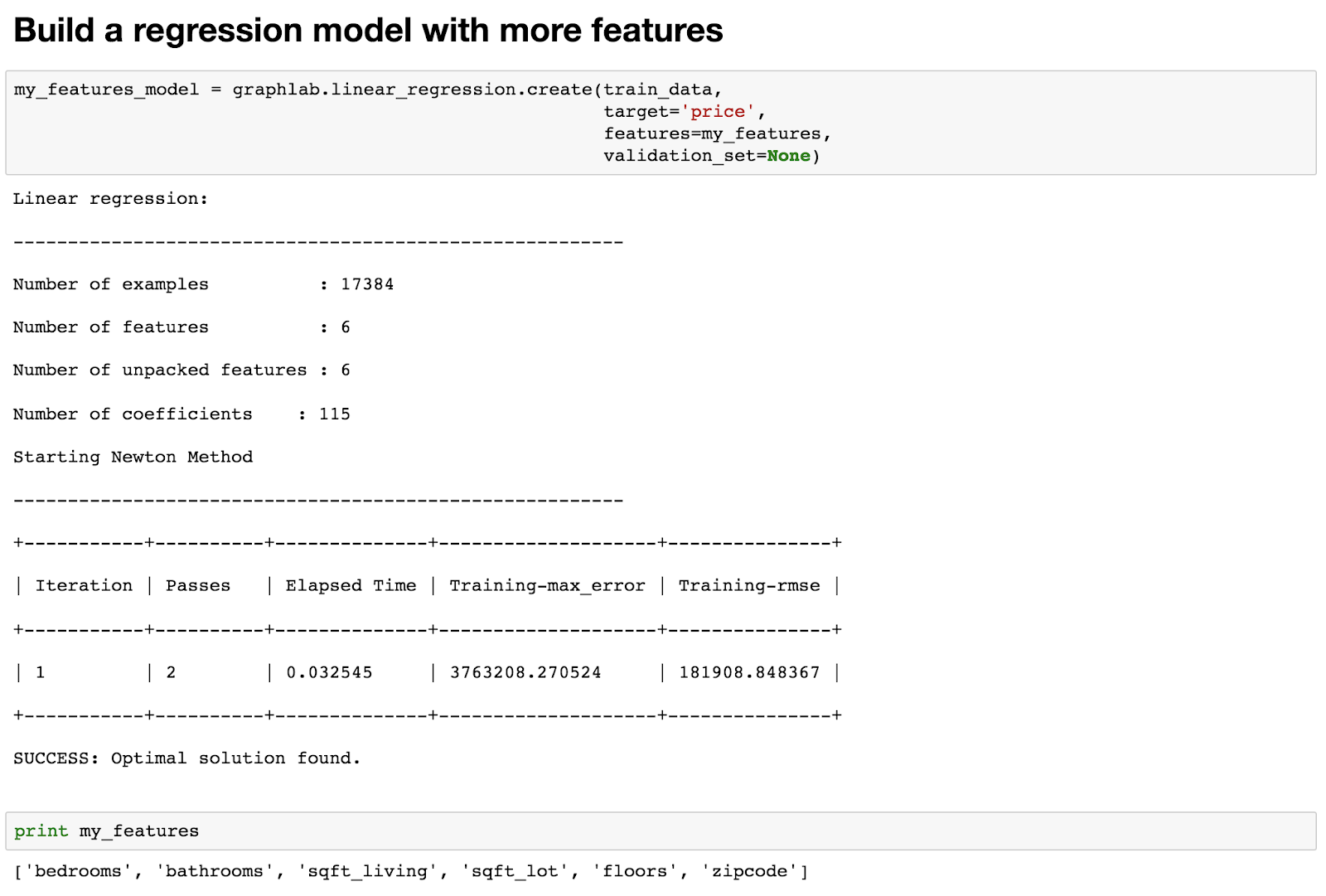
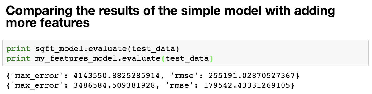
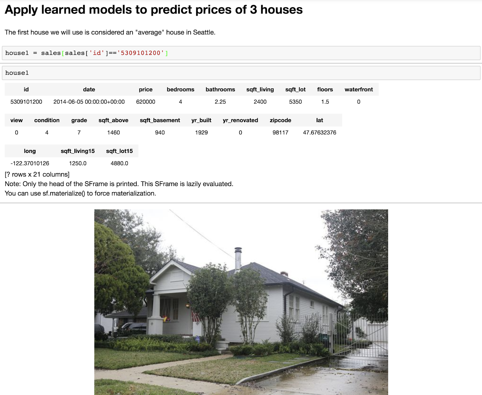
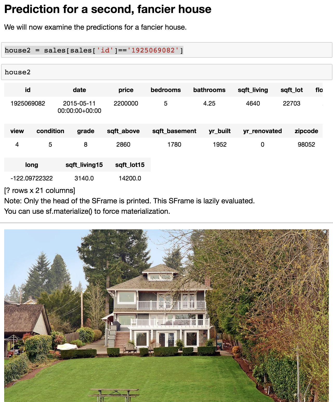
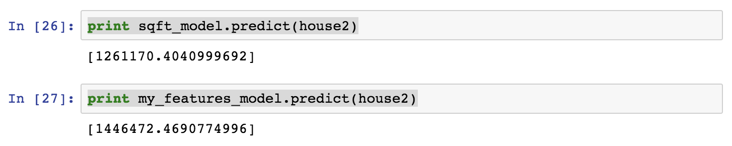
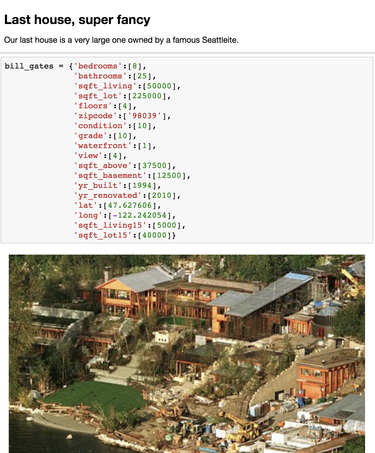
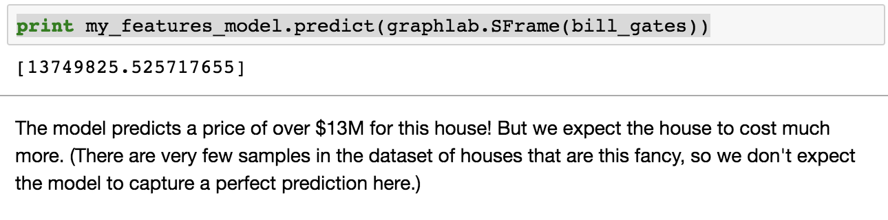
Machine Learning - Predicting House Prices : python Machine Learning with the tools IPython Notebook & GraphLab Machine Learning with the tools IPython Notebook & GraphLab Create on AWS Machine Learning with the tools IPython Notebook Usage Machine Learning with the tools IPython Notebook SFrame Machine Learning - Predicting House Prices : Regression 우리는 주택 가격을 예측하는 데 Regression 을 사용하는 방법에 대해 이야기 해보겠습니다. 이제 King County 데이터를 기반으로 실제 데이터 세트의 주택 가격을 예측하기 위해 Python을 사용하여 Jupyter Notebook을 구성하고 가격을 책정합니다. King County는 시애틀(Seattle)이 있는 지역입니다. 따라서 우리는 데이터 중 일부를 공개 기록 데이터(public record data)로 사용하고, 집값을 예측하기 위해 실제로 regression을 IPython notebook으로 구성합니다. 처음으로 graphlab create를 시작합니다. import graphlab 이제 우리의 임무는 집값을 예측하는 것입니다. 우리가 할 첫 번째 일은 주택 판매 데이터를 로드하는 것입니다. 이것은 시애틀 지역에서 판매 된 공공 데이터, 공공 기록입니다. sales = graphlab.SFrame(‘home_data.gl/’) 읽어온 데이터의 테이블을 sales라고 부를 것이며 graphlab .SFrame을 이용해 데이터를 가져옵니다. 우리는 graphlab에서 표 형식의 데이터를 표현하기 위한 데이터 구조로 SFrame에 대해 이야기했습니다. GraphLab Create를 실행하는 동안 입력 만하면 여기에 sales를 입력하면 해당 데이터가 어떻게 보이는지 알 수 있습니다. sales 데이터를 살펴보면, id와 date, 판매 가격, 침실의 수, 욕실의 수, 스퀘어 피트 등의 feature로 구성된 데이터가 있습니다. 우리가 할 첫 번째 일은 graph lab canvas를 사용하고 시각화(Visualization)를하는 것입니다. graphlab.canvas.set_target(‘ipynb’) .show()를 호출하면, 그 데이터의 시각화를 보여줄 것입니다. 분산형 플롯(Scatter plot)을 사용합니다. 우리는 두 변수를 관련시키는 plot을 생성할 것입니다. X 축에는 평방 피트의 생활 공간이 있습니다. y 축은 가격(price)이 됩니다. 우리는 가격의 평방 피트와의 관계를 확인할 것입니다. graphlab 캔버스에 기본 타겟 인 브라우저가 아니라 ipython notebook이 되도록 목표를 설정하도록 지시 할 수 있습니다. canvas.set_target ( 'ipynb'), ipython 노트북을 입력하면 notebook 자체 이 scatter plot이 표시합니다. 예를 들어, 평방 피트 큰 집으로 마우스를 올리면 plot에 대한 정보가 나옵니다. 5,790 평방 피트의 크기로 1,750,000 달러에 팔렸습니다. 백만 달러는 상당히 많은 돈입니다. 더 큰 주택에는 더 많은 비용이 드는 상관 관계가 있습니다. 가격을 1,000,000 달러 기준으로 평방 피트의 크기를 살펴보면, 일부 집 크기에 큰 평방 피트가 차이가 나지만, 가격은 거의 비슷한 경우가 생깁니다. train_data, test_data = sales.random_split(.8, seed=0) Regression Model을 생성하기 이전에 데이터셋을 train과 test로 split(분리) 합니다. 분리하는 방식은 여러가지가 있지만, random seed값을 부여하여 random으로 정해진 비율에 따라 split 할 수 있습니다. 첫 번째 parameter인 .8은 train을 80%로 test를 20%로 split 합니다. sqft_model = graphlab.linear_regression.create(train_data, Linear Regression 모델을 생성하기 위해 graphlab.linear_regression.create method를 호출합니다. 첫 번째 parameter로 model을 training 할 train_data, 2 번째로 예측할 변수(variable), 3 번째로 training할 feature, 4 번째로 뒤에서 배울 모델을 검증하는 방식인 validation_set 에 대해서 validation_data를 넣어야 합니다. print test_data['price'].mean() test_data의 가격(price)에 대한 평균값은 543,054 달러 입니다. Training을 시킨 model을 test_data로 평가해봅시다. evaluate method를 호출하여, test_data를 parameter로 넣습니다. print로 출력한 결과 max_error와 RMSE(Root Mean Squared Error) 값이 출력됩니다. import matplotlib.pyplot as plt 우리의 예측을 matplotlib을 이용해 도표로 표현해봅시다. matplotlib을 import로 불러오고, plt.plot method를 호출해 차트를 생성합니다. 우리가 그릴 것은 test data의 실제 sqft_living과 price를 . 점으로 표시하고, Linear Regression 모델에서 예측한 것을 -로 표기합니다. sqft_model.get('coefficients') 이번에는 Linear Regression 모델에서 coefficient(weight)를 가져옵니다. ^y = w1*x1 + w0 이며, w1은 sqft_living 이며, w0는 intercept 입니다. 각각의 value와 standard derivation(표준편차) 값을 확인할 수 있습니다. my_features = ['bedrooms', 'bathrooms', sales의 데이터셋에서 원하는 feature들만 가져와서 분포를 살펴봅니다. 각 feature들 마다 dtype(data type), num_unique(unique한 value의 개수), num_undefined(missing value), frequent_items(value 마다 개수)를 확인할 수 있으며, num_unique한 개수가 너무 많다면, min, max, median, mean, std 값을 확인할 수 있습니다. sales.show(view='BoxWhisker Plot', x='zipcode', y='price') 이번에는 다른 view로 feature들을 살펴보겠습니다. view는 BoxWhisker Plot으로 parameter를 설정하고, x축으로는 zipcode(우편번호), y축으로는 price(가격)을 넣습니다. 각 zipcode 별 가격을 살펴볼 수 있으며, 특정 zipcode 에 있는 집들의 가격이 높고 낮음을 확인 할 수 있습니다. my_features_model = graphlab.linear_regression.create(train_data, 위의 6개 feature를 이용해 Linear Regression 모델을 training 합니다. print sqft_model.evaluate(test_data) training을 한 2 개의 모델이 생성 되었습니다. 각 모델의 RMSE를 비교해봅시다. feature를 6개 사용한 모델의 RMSE가 더 낮은 것을 확인할 수 있습니다. 이번에는 3개의 집에 대해서 학습한 모델의 예측(prediction)을 살펴봅시다. house1 = sales[sales['id']=='5309101200'] 첫 번째 집은 sales 데이터에 특정 id를 부여하여 house1이라는 데이터로 넣습니다. house1에 대한 정보들을 살펴 볼 수 있습니다. 자 이제 실제 가격과 2개의 모델에서 예측한 가격을 비교해 봅시다. print house1['price'] 실제 가격은 620,000 달러이며, feature를 1개를 쓴 모델은 629,584 달러로 feature 6개를 쓴 모델 721,918 달러보다 잘 예측하였습니다. 그러나, 모델의 평균적인 예측에 있어서는 feature가 많은 모델이 더 낫습니다. 이번에는 house2에 대해 예측을 해봅시다. house2 = sales[sales['id']=='1925069082'] 각 2개의 모델에 예측 한 값을 살펴봅시다. print sqft_model.predict(house2) 실제 가격 2,200,000 에 비해 가격 예측을 잘 하지 못하였으나, feature 개수가 많은 모델이 좀 더 근접했습니다. 이번에는 Seattle에 있는 빌게이츠의 집에 대해서 직접 입력해봅시다. bill_gates = {'bedrooms':[8], 모델이 예측한 가격으로 테스트를 진행해봅시다. print my_features_model.predict(graphlab.SFrame(bill_gates) 이를 통해 우리는 집의 가격을 예측해보았습니다.출처 : Coursera / Emily Fox & Carlos Guestrin / Machine Learning Specialization / University of Washington
CreatePredicting House Prices
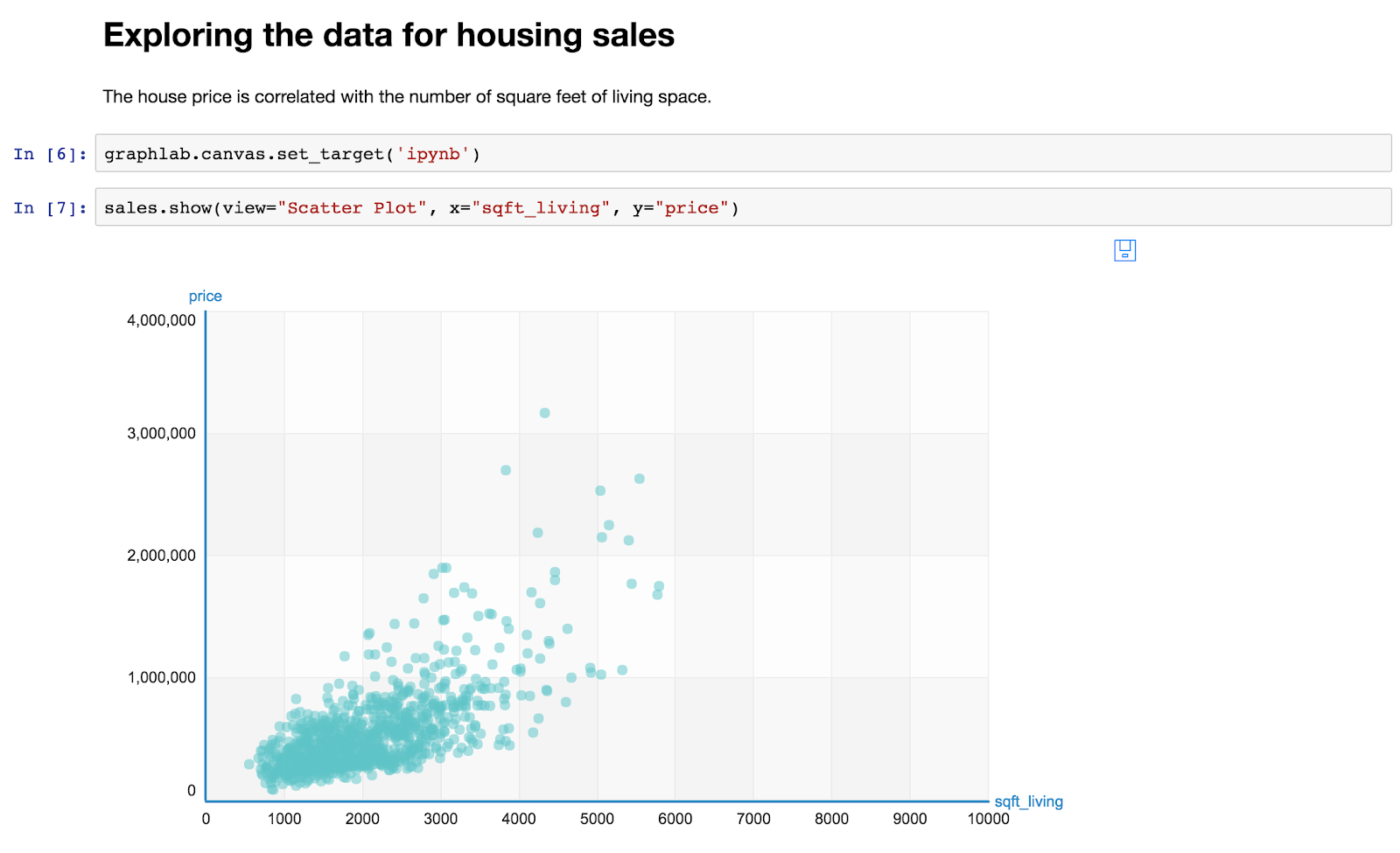
sales.show(view =“Scatter Plot”, x=“sqft_living”, y=“price”)
target='price',
features=['sqft_living'],
validation_set=None)
print sqft_model.evaluate(test_data)
%matplotlib inline
plt.plot(test_data['sqft_living'],test_data['price'],'.',
test_data['sqft_living'],sqft_model.predict(test_data),'-')
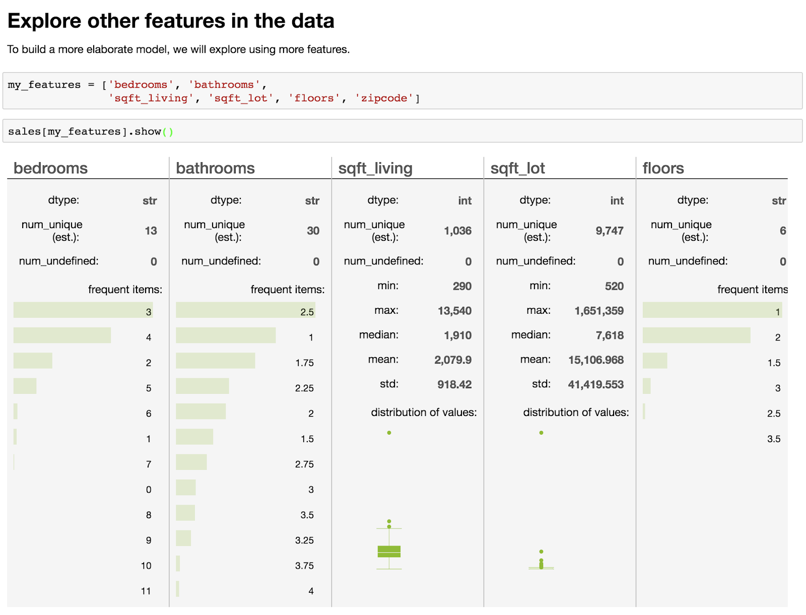
'sqft_living', 'sqft_lot', 'floors', 'zipcode']
sales[my_features].show()
target='price',
features=my_features,
validation_set=None)
print my_features
print my_features_model.evaluate(test_data)
house1
print sqft_model.predict(house1)
print my_feature_model.predict(house1)
house2
print my_features_model.predict(house2)
'bathrooms':[25],
'sqft_living':[50000],
'sqft_lot':[225000],
'floors':[4],
'zipcode':['98039'],
'condition':[10],
'grade':[10],
'waterfront':[1],
'view':[4],
'sqft_above':[37500],
'sqft_basement':[12500],
'yr_built':[1994],
'yr_renovated':[2010],
'lat':[47.627606],
'long':[-122.242054],
'sqft_living15':[5000],
'sqft_lot15':[40000]}


'MachineLearning' 카테고리의 다른 글
| Incorporating Field-aware Deep Embedding Networks and Gradient Boosting Decision Trees for Music Recommendation (0) | 2018.02.28 |
|---|---|
| Machine Learning - Classification : Analyzing Sentiment (0) | 2018.02.02 |
| Machine Learning - Predicting House Prices : Regression (0) | 2018.01.30 |
| Matrix Factorization Techniques for Recommender Systems (1) | 2018.01.04 |
| Spark MLlib ALS lastfm dataset (0) | 2017.11.28 |